CHAPTER 7: OPTIMAL RISKY PORTFOLIOS
CHAPTER 7: OPTIMAL RISKY PORTFOLIOS
PROBLEM SETS
1. (a) and (e). Short-term rates and labor issues are factors that are common to all
2. (a) and (c). After real estate is added to the portfolio, there are four asset classes in
the portfolio: stocks, bonds, cash, and real estate. Portfolio variance now includes a
4. The parameters of the opportunity set are:
From the standard deviations and the correlation coefficient we generate the
covariance matrix [note that
( , )
S B S B
Cov r r r s s= ´ ´
]:
Bonds Stocks
Bonds
225
45
Stocks 45 900
The minimum-variance portfolio is computed as follows:
wMin(S) =
1739.0
)452(225900
45225
)(Cov2
)(Cov
22
2
BSBS
BSB
,rr
,rr
The minimum variance portfolio mean and standard deviation are:
7-1
CHAPTER 7: OPTIMAL RISKY PORTFOLIOS
σ
Min =
2/12222
)],(Cov2[
BSBSBBSS
rrwwww
5.
Proportion
in Stock Fund
Proportion
in Bond Fund
Expected
Return
Standard
Deviation
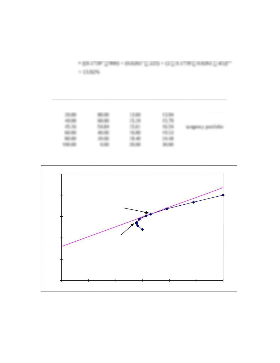
0.00% 100.00% 12.00% 15.00%
17.39 82.61 13.39 13.92 minimum variance
Graph shown below.
0.00
5.00
10.00
15.00
20.00
25.00
0.00
5.00
10.00
15.00
20.00
25.00
30.00
Tangency
Portfolio
Minimum
Variance
Portfolio
Efficient frontier
of risky assets
CML
INVESTMENT OPPORTUNITY SET
rf = 8.00
6. The above graph indicates that the optimal portfolio is the tangency portfolio with
expected return approximately 15.6% and standard deviation approximately 16.5%.
7-2
CHAPTER 7: OPTIMAL RISKY PORTFOLIOS
7-3
CHAPTER 7: OPTIMAL RISKY PORTFOLIOS
7. The proportion of the optimal risky portfolio invested in the stock fund is given by:
2
2 2
[ ( ) ] [ ( ) ] ( , )
[ ( ) ] [ ( ) ] [ ( ) ( ) ] ( , )
S f B B f S B
S
S f B B f S S f B f S B
E r r E r r Cov r r
wE r r E r r E r r E r r Cov r r
s
s s
– ´ – – ´
=– ´ + – ´ – – + – ´
[(.20 .08) 225] [(.12 .08) 45] 0.4516
[(.20 .08) 225] [(.12 .08) 900] [(.20 .08 .12 .08) 45]
– ´ – – ´
= =
– ´ + – ´ – – + – ´
1 0.4516 0.5484
B
w= – =
The mean and standard deviation of the optimal risky portfolio are:
8. The reward-to-volatility ratio of the optimal CAL is:
( ) .1561 .08 0.4601
.1654
p f
p
E r r
s
––
= =
9. a. If you require that your portfolio yield an expected return of 14%, then you
can find the corresponding standard deviation from the optimal CAL. The
equation for this CAL is:
( )
( ) .08 0.4601
p f
C f C C
P
E r r
E r r s s
s
–
= + = +
If E(rC) is equal to 14%, then the standard deviation of the portfolio is
13.04%.
b. To find the proportion invested in the T-bill fund, remember that the mean of
the complete portfolio (i.e., 14%) is an average of the T-bill rate and the
optimal combination of stocks and bonds (P). Let y be the proportion invested
in the portfolio P. The mean of any portfolio along the optimal CAL is:
( ) (1 ) ( ) [ ( ) ] .08 (.1561 .08)
C f P f P f
E r y r y E r r y E r r y= – ´ + ´ = + ´ – = + ´ –
Setting E(rC) = 14% we find: y = 0.7884 and (1 − y) = 0.2119 (the proportion
invested in the T-bill fund).
7-4
CHAPTER 7: OPTIMAL RISKY PORTFOLIOS
7-5
CHAPTER 7: OPTIMAL RISKY PORTFOLIOS
10. Using only the stock and bond funds to achieve a portfolio expected return of 14%,
we must find the appropriate proportion in the stock fund (wS) and the appropriate
proportion in the bond fund (wB = 1 − wS) as follows:
This is considerably greater than the standard deviation of 13.04% achieved using
T-bills and the optimal portfolio.
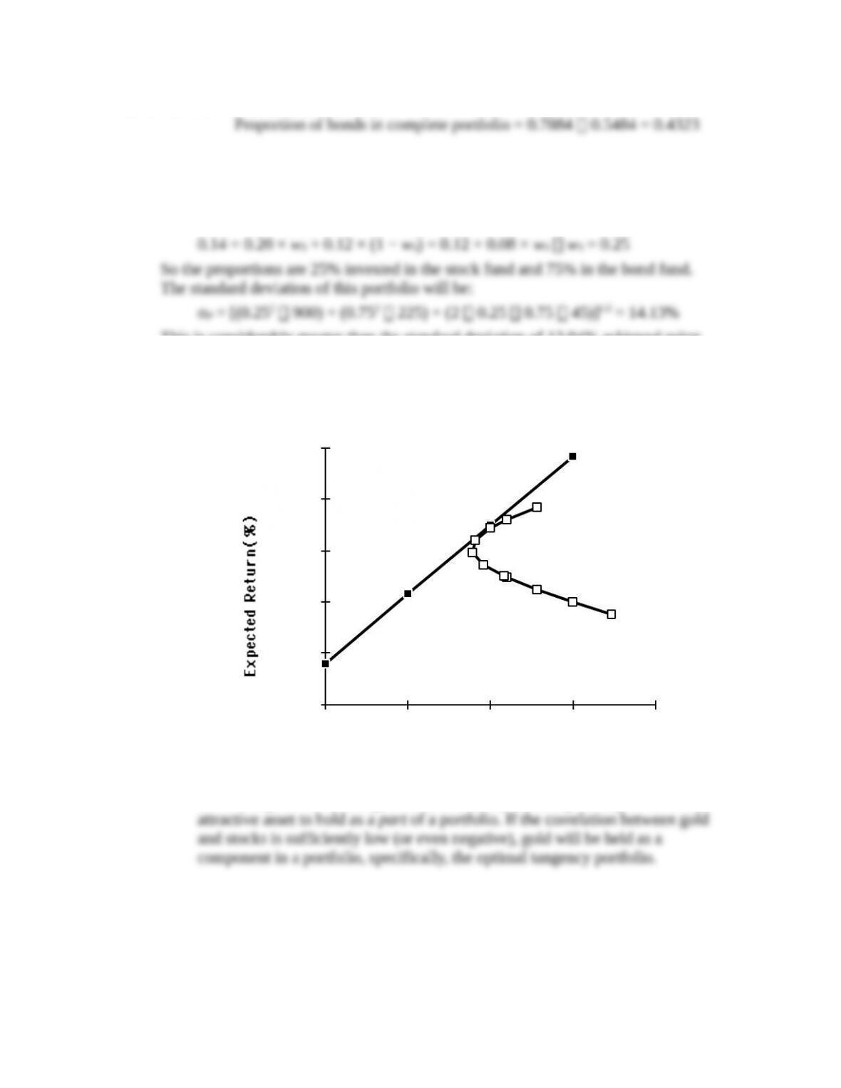
11. a.
Standar d Deviat ion(% )
0.00
5.00
10.00
15.00
20.00
25.00
0 10 20 30 40
Gold
Stocks
Optim al CAL
P
Even though it seems that gold is dominated by stocks, gold might still be an
7-6
CHAPTER 7: OPTIMAL RISKY PORTFOLIOS
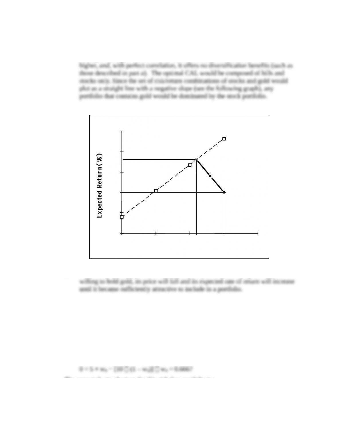
b. If the correlation between gold and stocks equals +1, then no one would be
willing to hold gold: its return is lower than stocks, its standard deviation is
Standard Deviation(%)
0
5
10
15
20
25
0.00
10.00
20.00
30.00
40.00
Gold
Stocks
r
f
18
c. Of course, this situation could not be an equilibrium. As long as no one is
12. Since Stock A and Stock B are perfectly negatively correlated, a risk-free portfolio
can be created and the rate of return for this portfolio, in equilibrium, will be the
risk-free rate. To find the proportions of this portfolio [with the proportion wA
invested in Stock A and wB = (1 – wA ) invested in Stock B], set the standard
deviation equal to zero. With perfect negative correlation, the portfolio standard
deviation is:
σP = Absolute value [wAσA wBσB]
The expected rate of return for this risk-free portfolio is:
7-7

CHAPTER 7: OPTIMAL RISKY PORTFOLIOS
Therefore, the risk-free rate is: 11.667%
7-8
CHAPTER 7: OPTIMAL RISKY PORTFOLIOS
of the component-asset standard deviations. The portfolio variance is a weighted
sum of the elements in the covariance matrix, with the products of the portfolio
proportions as weights.
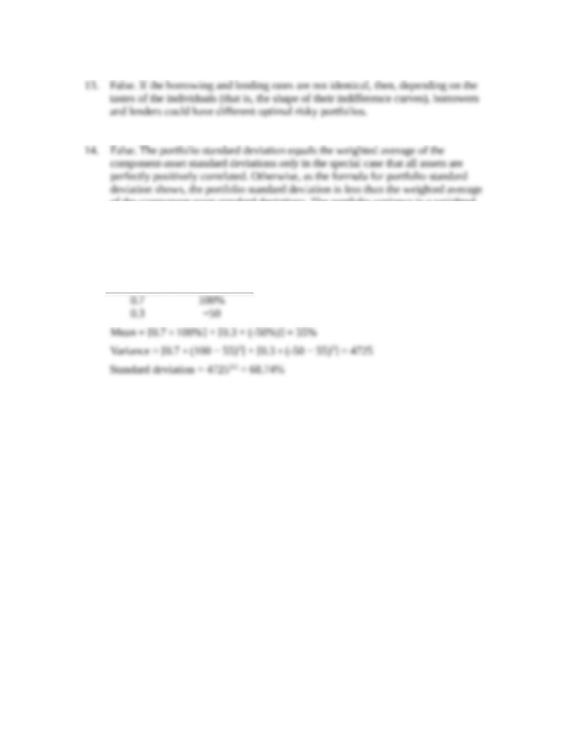
15. The probability distribution is:
Probability Rate of Return
7-9