CHAPTER 24: PORTFOLIO PERFORMANCE EVALUATION
CHAPTER 24: PORTFOLIO PERFORMANCE EVALUATION
PROBLEM SETS
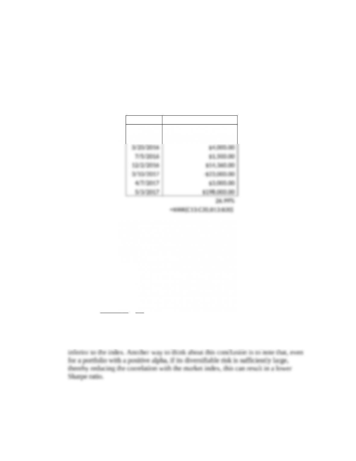
1. The dollar-weighted average will be the internal rate of return between the initial and
final value of the account, including additions and withdrawals. Using Excel’s XIRR
function, utilizing the given dates and values, the dollar-weighted average return is as
follows:
Date Account
1/1/2016 -$148,000.00
1/3/2016 $2,500.00
Since the dates of additions and withdrawals are not equally spaced, there really is no
way to solve this problem using a financial calculator. Excel can solve this very
quickly.
2. As established in the following result from the text, the Sharpe ratio depends on both
alpha for the portfolio (
P
a
) and the correlation between the portfolio and the market
index (ρ):
( ) αρ
σ σ
P f P
M
P P
E r r S
–= +
Specifically, this result demonstrates that a lower correlation with the market index
reduces the Sharpe ratio. Hence, if alpha is not sufficiently large, the portfolio is
3. The IRR (i.e., the dollar-weighted return) cannot be ranked relative to either the
geometric average return (i.e., the time-weighted return) or the arithmetic average
24-1
CHAPTER 24: PORTFOLIO PERFORMANCE EVALUATION
return. Under some conditions, the IRR is greater than each of the other two averages,
and similarly, under other conditions, the IRR can also be less than each of the other
averages. A number of scenarios can be developed to illustrate this conclusion. For
4. It is not necessarily wise to shift resources to timing at the expense of security
selection. There is also tremendous potential value in security analysis. The decision as
Stock XYZ has greater dispersion.
(Note: We used 5 degrees of freedom in calculating standard deviations.)
c. Geometric average:
Despite the fact that the two stocks have the same arithmetic average, the
e. Even though the dispersion is greater, your expected rate of return would
still be the arithmetic average, or 10%.
f. In terms of “forward-looking” statistics, the arithmetic average is the
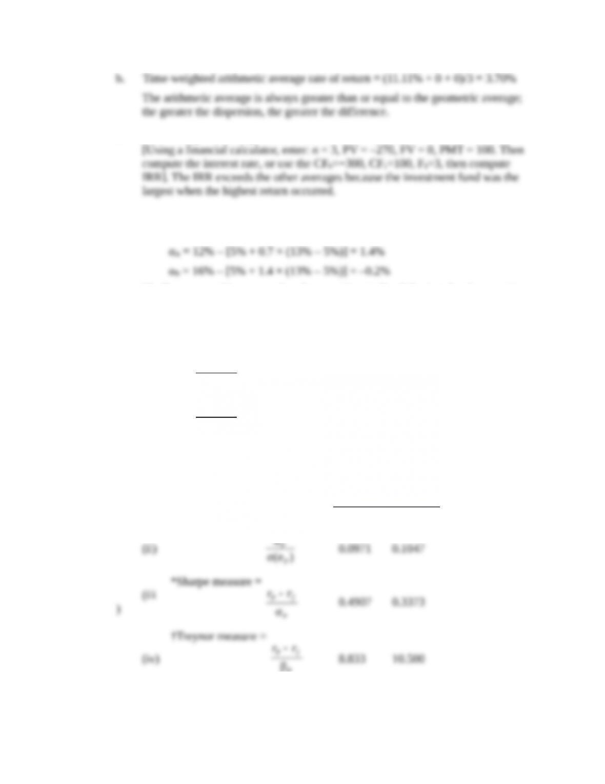
6. a. Time-weighted average returns are based on year-by-year rates of return:
24-2
CHAPTER 24: PORTFOLIO PERFORMANCE EVALUATION
Year Return = (Capital gains + Dividend)/Price
2016 − 2017
[($120 – $100) + $4]/$100 = 24.00%
2017 – 2018 [($90 – $120) + $4]/$120 = –21.67%
2018 − 2019 [($100 – $90) + $4]/$90 = 15.56%
Arithmetic mean: (24% – 21.67% + 15.56%)/3 = 5.96%
Geometric mean: (1.24 × 0.7833 × 1.1556)1/3 – 1 = 0.0392 = 3.92%
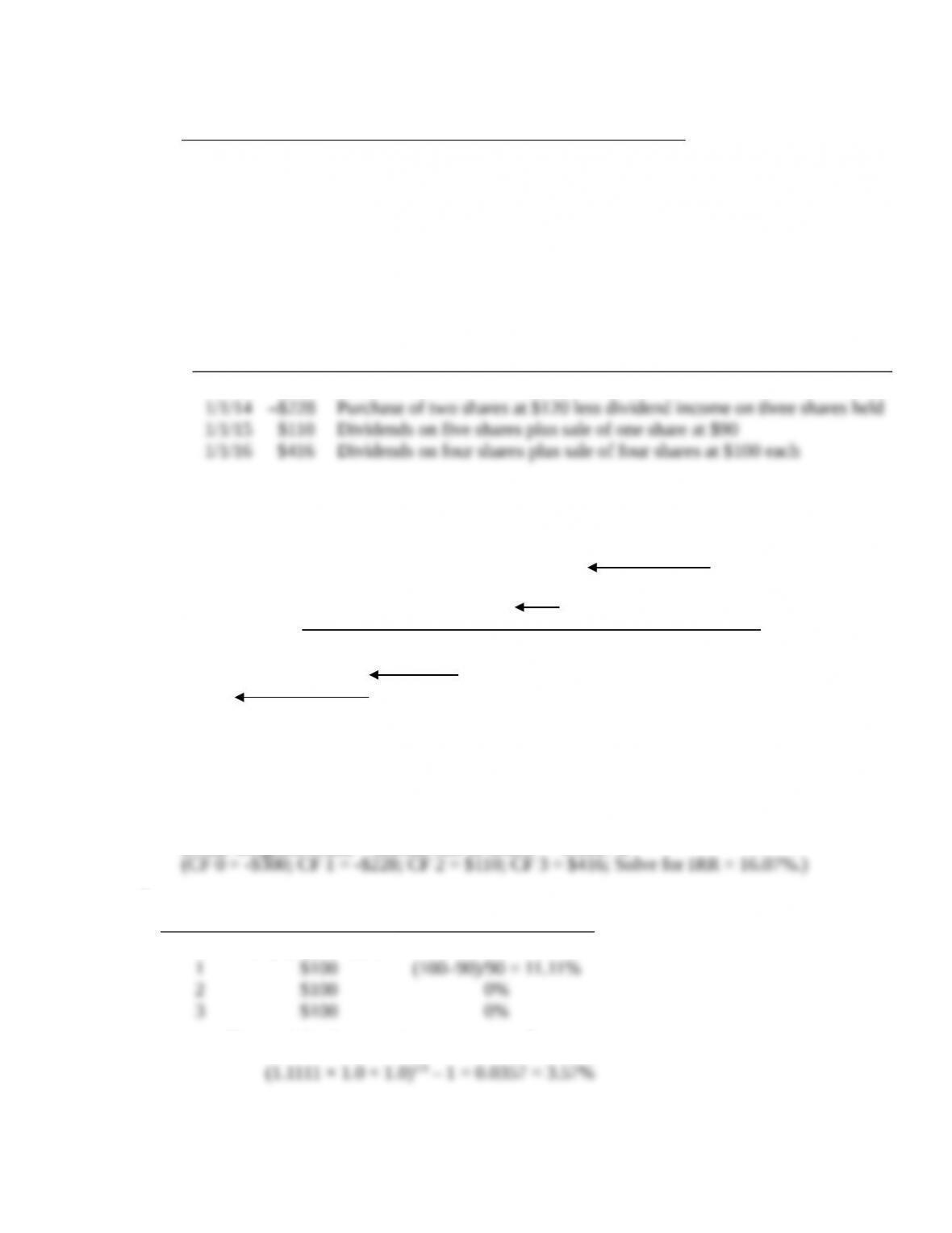
b.
Date
Cash
Flow Explanation
1/1/13 –$300 Purchase of three shares at $100 each
416
110
Date: 1/1/13 1/1/14 1/1/15 1/1/16
228
300
Dollar-weighted return = Internal rate of return = –0.1607%
7.
Time Cash Flow Holding Period Return
0 3×(–$90) = –$270
a. Time-weighted geometric average rate of return =
24-3
CHAPTER 24: PORTFOLIO PERFORMANCE EVALUATION
c. Dollar-weighted average rate of return = IRR = 5.46%
8. a. The alphas for the two portfolios are:
Ideally, you would want to take a long position in Portfolio A and a short position
in Portfolio B.
b. If you will hold only one of the two portfolios, then the Sharpe measure is the
appropriate criterion:
.12 .05 0.583
.12
A
S–
= =
.16 .05 0.355
.31
B
S–
= =
Using the Sharpe criterion, Portfolio A is the preferred portfolio.
9.
a. Stock A Stock B
(i) Alpha = regression intercept 1.0% 2.0%
Information ratio =
α
P
β
P
24-4
CHAPTER 24: PORTFOLIO PERFORMANCE EVALUATION
* To compute the Sharpe measure, note that for each stock, (rP – rf ) can be
computed from the right-hand side of the regression equation, using the assumed
† The beta to use for the Treynor measure is the slope coefficient of the
regression equation presented in the problem.
b. (i) If this is the only risky asset held by the investor, then Sharpe’s measure is the
(ii) If the stock is mixed with the market index fund, then the contribution to the
(iii) If the stock is one of many stocks, then Treynor’s measure is the
10. We need to distinguish between market timing and security selection abilities. The
intercept of the scatter diagram is a measure of stock selection ability. If the
Timing ability is indicated by the curvature of the plotted line. Lines that become
steeper as you move to the right along the horizontal axis show good timing ability.
We can therefore classify performance for the four managers as follows:
Selection
Ability Timing Ability
A. Bad Good
24-5
CHAPTER 24: PORTFOLIO PERFORMANCE EVALUATION
b. Security Selection:
(1) (2) (3) = (1) × (2)
Market
Differential Return
within Market
(Manager – Index)
Manager’s
Portfolio
Weight
Contribution to
Performance
Equity –0.5% 0.70 −0.35%
c. Asset Allocation:
(1) (2) (3) = (1) × (2)
Market
Excess Weight
(Manager – Benchmark)
Index
Return
Contribution to
Performance
Equity 0.10% 2.5% 0.25%
Summary:
b. Added value from country allocation:
(1) (2) (3) = (1) × (2)
Country Excess Weight
(Manager – Benchmark)
Index Return
minus Bogey
Contribution to
Performance
U.K. 0.15 −1.8% −0.27%
c. Added value from stock selection:
(1) (2) (3) = (1) × (2)
Differential Return
within Country Manager’s Contribution to
24-6
CHAPTER 24: PORTFOLIO PERFORMANCE EVALUATION
Country (Manager – Index) Country
weight Performance
U.K. 0.08 0.30% 2.4%
Summary:
13. Support: A manager could be a better performer in one type of circumstance than in
another. For example, a manager who does no timing but simply maintains a high beta, will
Contradict: If we adequately control for exposure to the market (i.e., adjust for beta),
14. The use of universes of managers to evaluate relative investment performance does,
b. From Black-Jensen-Scholes and others, we know that, on average, portfolios
with low beta have historically had positive alphas. (The slope of the empirical
16. a. The most likely reason for a difference in ranking is due to the absence of
diversification in Fund A. The Sharpe ratio measures excess return per unit of
24-7
CHAPTER 24: PORTFOLIO PERFORMANCE EVALUATION
17. The within sector selection calculates the return according to security selection. This is
done by summing the weight of the security in the portfolio multiplied by the return of
the security in the portfolio minus the return of the security in the benchmark:
Large Cap Sector: 0.6 (.17-.16)= 0.6%
Mid Cap Sector: 0.15 (.24 –.26) -0.3%
Small Cap Sector: 0.25 (.20-.18)= 0.5%
Total Within-Sector Selection = 0.6% – 0.3% 0.5% 0.8%
´
´ =
´
+ =
18. Primo Return
0.6 17% 0.15 24% 0.25 20% 18.8%= ´ + ´ + ´ =
Benchmark Return
0.5 16% 0.4 26% 0.1 18% 20.2%= ´ + ´ + ´ =
Primo – Benchmark = 18.8% − 20.2% = -1.4% (Primo underperformed benchmark)
To isolate the impact of Primo’s pure sector allocation decision relative to the
benchmark, multiply the weight difference between Primo and the benchmark
portfolio in each sector by the benchmark sector returns:
(0.6 0.5) (.16) (0.15 0.4) (.26) (0.25 0.1) (.18) 2.2%– ´ + – ´ + – ´ =-
To isolate the impact of Primo’s pure security selection decisions relative to the
benchmark, multiply the return differences between Primo and the benchmark for each
sector by Primo’s weightings:
(.17 .16) (.6) (.24 .26) (.15) (.2 0.18) (.25) 0.8%– ´ + – ´ + – ´ =
19. Because the passively managed fund is mimicking the benchmark, the
2
R
of the
20. a. The euro appreciated while the pound depreciated. Primo had a greater stake in
the euro-denominated assets relative to the benchmark, resulting in a positive

CHAPTER 24: PORTFOLIO PERFORMANCE EVALUATION
24-9