5699.0 2
2
0=+=
DDD CCC
DD CC
Problem 14 – It is desired to develop a close protection system using a 0.50 caliber machine gun.
The muzzle velocity of the weapon is 2,950 ft/s. The projectile is an M8 bullet with a diameter
of 0.50 in. and a mass of 0.09257 lbm. Since the projectile interception mission is to occur
relatively close to the firing platform we can assume the projectile behaves according to the flat
fire assumption with a constant drag coefficient of K1 = 0.45 [unitless]. Assuming the flat fire
assumption is valid for the trajectory and the intercept point is to be 20 ft above the ground,
develop a firing table for the intercept out to 300 yards in 50 yard increments. Assume standard
sea level met data (
= 0.0751 lbm/ft3, a = 1,120 ft/s,
( )
−
−
=Rslug
lbfft
716,1R
)
Create a table containing range (yards), impact velocity (ft/s), time of flight (s), and initial
quadrant elevation angle (degrees) in 50 yard increments out to 300 yards. Comment on the
accuracy of your answer.
1== KCD
We can now calculate k1 from equation (FF-50)
( ) ( )
( )( )
( )
=
== −
ft
1
10489.245.0
lbm09257.02
ft001364.0
ft
lbm
0751.0
2
4
2
3
11 K
m
S
k
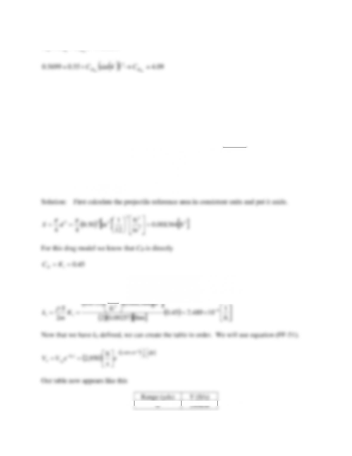
Now that we have k1 defined, we can create the table in order. We will use equation (FF-51).
( )
( )
ft
ft
1
10489.2 4
1
0s
ft
950,2
x
xk
xx eeVV
−
−
−
==
Our table now appears like this
Range (yds)
V (ft/s)
0
2950.0

50
2841.9
100
2737.7
150
2637.4
200
2540.8
250
2447.7
300
2358.0
Now that we have the impact velocity we can obtain the time of flight from equation (FF-53).
( )
( )
( )
( )
−
=−=
−
−
1
ft
1
10489.2
s
ft
950,2
1
1
1ft
ft
1
10489.2
4
1
4
1
0
x
xk
x
ee
kV
t
The table is now
Range
(yards)
V
(ft/s)
t
(seconds)
0
2950.0
0.00
50
2841.9
0.05
100
2737.7
0.11
150
2637.4
0.16
200
2540.8
0.22
250
2447.7
0.28
300
2358.0
0.34
The elevation angle of the weapon is determined by solving equation (FF-57) for
0 with y0 set
equal to zero and y set equal to 20 ft. Thus we have
( )
( )
( )
( )
( )
ft
s
ft
1
10489.2
s
ft
950,2
s
ft
1
10489.2
s
ft
950,2
2
ft2
tan 2
4
4
0x
t
t
x
+
−
+
=
−
−
Range
(yards)
V
(ft/s)
t (seconds)
0
(degrees)
0
2950.0
0.00
–
50
2841.9
0.05
21.84
100
2737.7
0.11
11.41
150
2637.4
0.16
7.75
200
2540.8
0.22
5.92
250
2447.7
0.28
4.84
300
2358.0
0.34
4.15
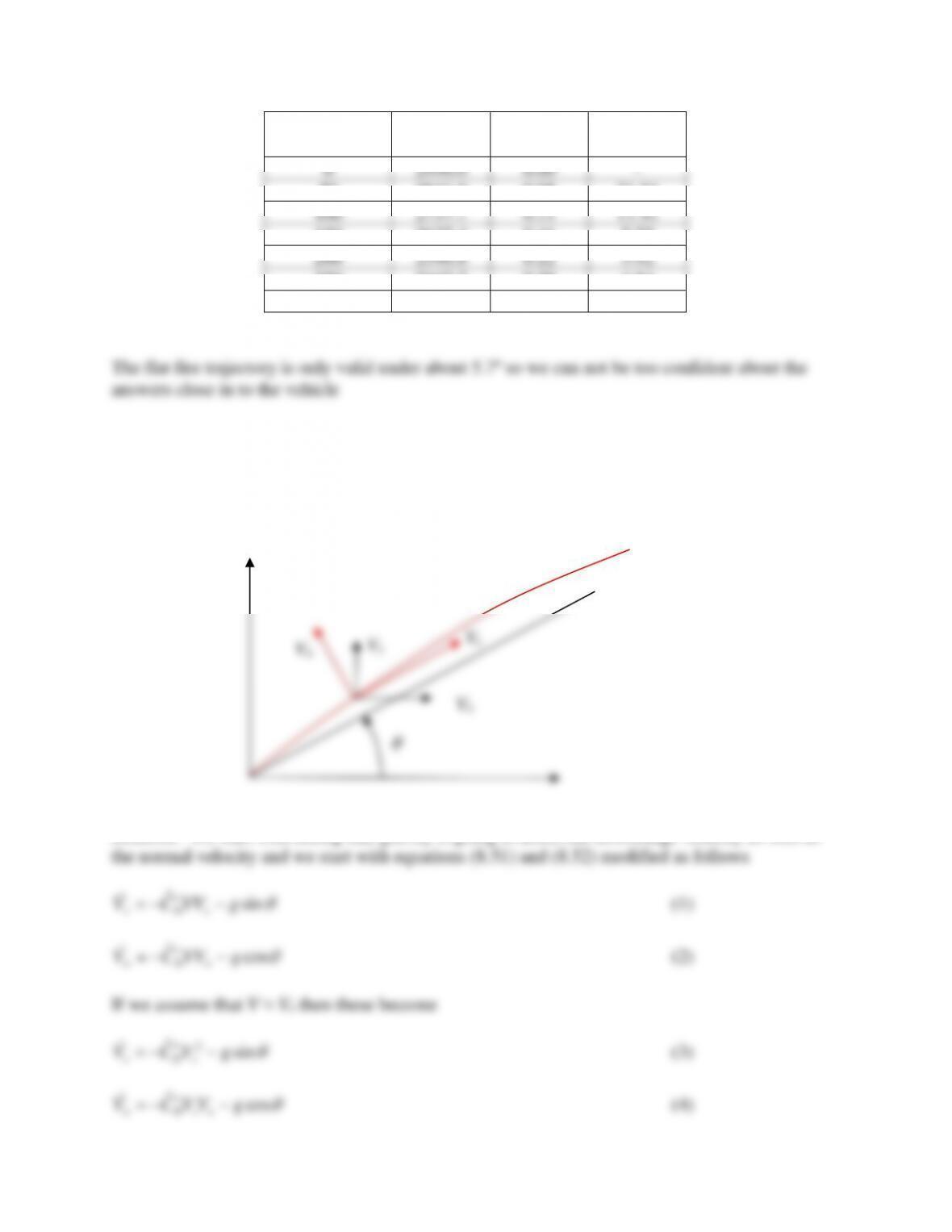
Problem 15 – If we were to assume that the flat fire conditions were to hold in a coordinate
system that were elevated to an angle θ, re-derive the differential equations in time an space
coordinates – DO NOT solve them, just put them in the form of equations (8.60) and (8.61).
Also write the transformation equations between the normal and slant velocity (Vn and Vs) and Vx
and Vy.
Solution: We start with noting that gravity is going to affect the downrange velocity as well as
θ
Vx
Vy
Vs
Vn
Making the coordinate transformations from time to distance we have
ns
s
nVV
ds
dt
ds
dt
Substituting this back into equations (3) and (4) yields
s
nDn V
Finally, the transformation equations between the slant velocities and the true velocities are
Problem 16 – One of the problems with hit-to-kill close protection systems is the ability to
accurately point the weapon and fire in a timely fashion at a very small target. Assume that we
must impact a sphere 4 inches in diameter at the ranges developed in problem 14. For each
range, assuming perfect timing as well as perfect projectile tracking, determine the allowable
tolerance in Q.E. to impact the target.
( )
( )
( )
( )
( )
( )
( )
( )
( )
ft
ft167.20
s
ft
1
10489.2
s
ft
950,2
s
ft
1
10489.2
s
ft
950,21ln
s
ft
1
10489.2
s
ft
950,2
1
2
1
ft2
s
s
ft
2.32
tan 2
4
4
4
22
2
0x
t
t
t
x
t
+
+
−
+
=
−
−
−
Range
(yards)
V
(ft/s)
t (seconds)
0
(degrees)
’0
(degrees)
0
2950.0
0.00
–
–
50
2841.9
0.05
21.84
22.01
100
2737.7
0.11
11.41
11.50
150
2637.4
0.16
7.75
7.81
200
2540.8
0.22
5.92
5.97
250
2447.7
0.28
4.84
4.88
300
2358.0
0.34
4.15
4.18
( )
( )
( )
( )
( )
( )
( )
( )
( )
ft
ft83.19
s
ft
1
10489.2
s
ft
950,2
s
ft
1
10489.2
s
ft
950,21ln
s
ft
1
10489.2
s
ft
950,2
1
2
1
ft2
s
s
ft
2.32
tan 2
4
4
4
22
2
0x
t
t
t
x
t
+
+
−
+
=
−
−
−
Range
(yards)
V
(ft/s)
t (seconds)
0
(degrees)
’0
(degrees)
”0
(degrees)
0
2950.0
0.00
–
–
–
50
2841.9
0.05
21.84
22.01
21.68
100
2737.7
0.11
11.41
11.50
11.31
150
2637.4
0.16
7.75
7.81
7.68
200
2540.8
0.22
5.92
5.97
5.87
250
2447.7
0.28
4.84
4.88
4.81
300
2358.0
0.34
4.15
4.18
4.11
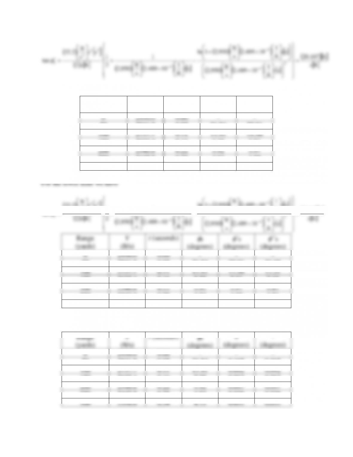
The upper and lower limits in degrees are then
Range
(yards)
V
(ft/s)
t (seconds)
0
(degrees)
+
(degrees)
–
(degrees)
0
2950.0
0.00
–
–
–
50
2841.9
0.05
21.84
0.165
0.165
100
2737.7
0.11
11.41
0.092
0.092
150
2637.4
0.16
7.75
0.063
0.063
200
2540.8
0.22
5.92
0.047
0.047
250
2447.7
0.28
4.84
0.038
0.038
300
2358.0
0.34
4.15
0.032
0.032
Problem 17 – Let’s now assume that the pointing against the incoming round in problem 14 is
absolutely perfect. Determine the tolerance in lock time (officially the time from pulling the
trigger to weapon firing – but we’ll assume it is to muzzle exit) to hit the target at the conditions
of problem 14. Assume that the incoming projectile is moving at 300 ft/s. How does this change
if the velocity estimate is ± 20 ft/s?
Problem 18 – The main armament of the last Pre-war U.S. Heavy Cruisers (known as the “tin–
clads”) was an 8”/55 cal weapon. The effective range of this weapon was 30,000 yards at an
elevation of 40º43’. During the Second World War there were many night actions in the pacific
where these weapons were used at an extremely short range (less than 10,000 yards). You are
asked to create a firing table for this weapon at the short ranges. The muzzle velocity of the
weapon/projectile/propellant combination is 2,500 ft/s. The projectile is an APC (Armor
Piercing, Capped) with a diameter of 8 in. and a mass of 335 lbm. Since the range is short we
can assume the projectile behaves according to the flat fire assumption with a drag coefficient
inversely proportional to the Mach number of K2 = 0.62 [unitless] (note that this is not really a
great fit for this projectile). Assuming the flat fire assumption is valid for the trajectory, develop
a firing table for the system to 10,000 yards in 1,000 yard increments. Assume standard sea level
met data (
= 0.0751 lbm/ft3, a = 1,120 ft/s,
( )
−
−
=Rslug
lbfft
716,1R
)
Create a table containing range (yards), impact velocity (ft/s), time of flight (s), and initial
quadrant elevation angle (degrees) in 1,000 yard increments out to 10,000 yards.
Solution:
0−=
Our table now appears like this
Range (yards)
V (ft/s)
0
2500
1000
2418
2000
2337
3000
2255
4000
2174
5000
2092
6000
2011
7000
1929
8000
1848
9000
1766
10000
1685
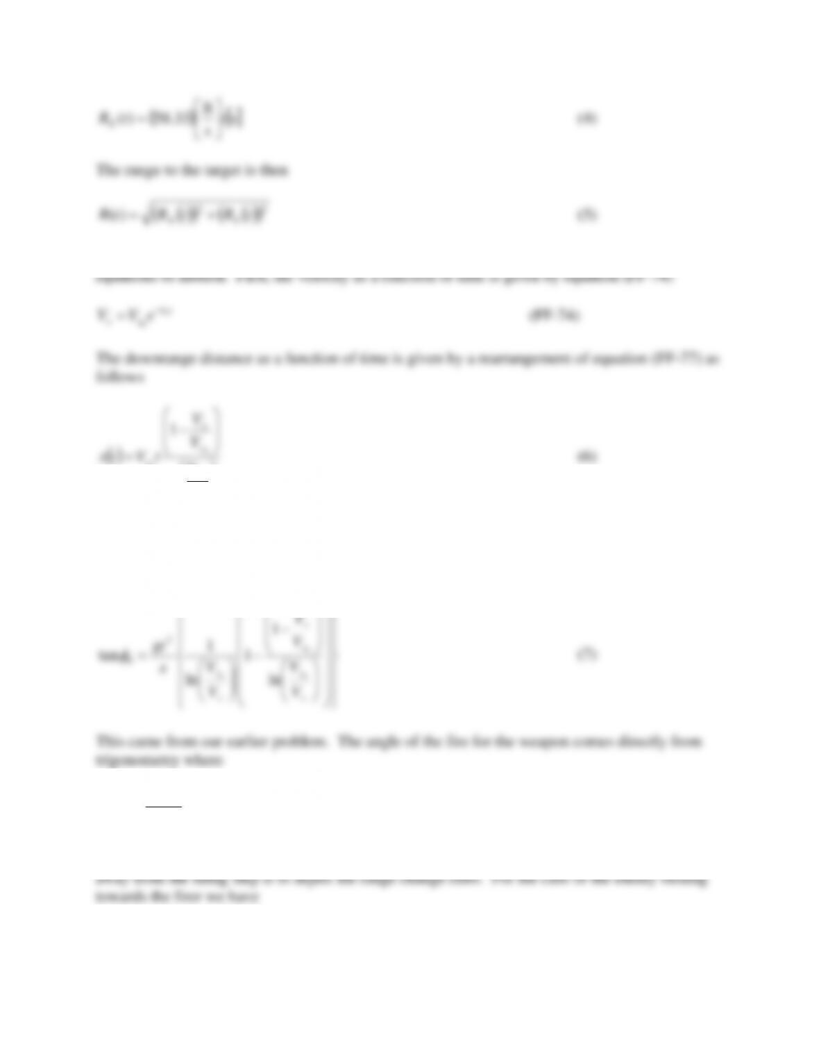
Now that we have the impact velocity we can obtain the time of flight from equation (FF-77).
−
=
0
0
01
ln
x
x
x
x
x
V
V
V
V
V
x
t
(FF-77)
The table is now
Range
(yards)
V
(ft/s)
t
(seconds)
0
2500
0.00
1000
2418
1.22
2000
2337
2.48
3000
2255
3.79
4000
2174
5.14
5000
2092
6.55
6000
2011
8.01
7000
1929
9.53
8000
1848
11.12
9000
1766
12.78
10000
1685
14.52
The elevation angle of the weapon is determined by solving equation (FF-85) for
0 with y and y0
set equal to zero. Thus we have
x
x
x
x
x
x
x
x
V
V
V
V
x
V
V
V
V
0
00
0ln
ln
ln
ln
2
0
00
Using the above relation we obtain the angle multiply this by 60 to obtain the angle in minutes.
Range
(yards)
V
(ft/s)
t (seconds)
0
(minutes)
0
2500
0.00
–
1000
2418
1.22
27
2000
2337
2.48
56
3000
2255
3.79
85
4000
2174
5.14
116
5000
2092
6.55
149
6000
2011
8.01
184
7000
1929
9.53
220
8000
1848
11.12
258
9000
1766
12.78
299
10000
1685
14.52
341
For the final task of part b) we calculate the angle of fall from equation (FF-81) below
−
−
+=
0
0
01
1
tantan 2
0
x
x
x
x
x
V
V
V
V
V
gx
(FF-81)
Inserting the data from the table yields the final result
Range
(yards)
V
(ft/s)
t (seconds)
0
(minutes)
(minutes)
0
2500
0.00
–
–
1000
2418
1.22
27
-28
2000
2337
2.48
56
-58
3000
2255
3.79
85
-91
4000
2174
5.14
116
-128
5000
2092
6.55
149
-168
6000
2011
8.01
184
-212
7000
1929
9.53
220
-261
8000
1848
11.12
258
-316
9000
1766
12.78
299
-376
10000
1685
14.52
341
-443
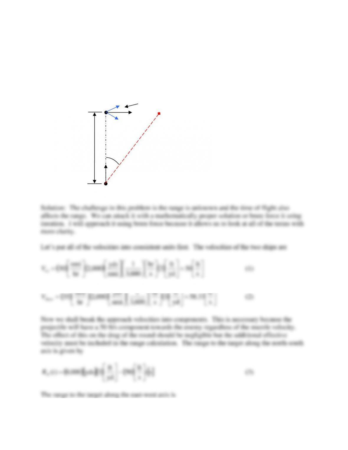
Problem 19 – The analog fire control computers installed on board ships during the Second
World War were amazing devices. The inputs required were course and speed of the firing ship,
estimated range to the target and course and speed of the target. Inaccuracies in the target course
and speed estimates were compensated for by generating a “ladder” this was a shell pattern that
was a linear array using as many guns as were available in one “salvo”. The ideal result was that
the target would end up directly in the middle of the “salvo” and be “straddled”. Because of the
relatively flat projection of the shells, being straddled usually guaranteed that the target was hit
by at least one projectile. The shorter the range to a target, the larger the “danger space” offered
and the better the chance of a hit. In this problem you assume the role of the fire control
computer. The weapons available are nine 8”/55 caliber guns with the ballistic performance
from problem 18. Your ship is moving due north at 30 knots (one Knot is one nautical mile per
hour or 2000 yards per 3600 seconds). At the instant of fire, the enemy ship is dead ahead of
your ship traveling at 35 knots on course 090 (see the figure) at a range of 8,000 yards. Ignore
the effect of the launch platform motion on the drag (only) of the projectile
a.) Determine the firing solution assuming both ships continue straight ahead (Q.E. and
relative angle to the bow of your ship) for one shell to impact the enemy (Because of the flat
trajectory it’s good to aim so the shell falls a little behind the enemy ship) – Hint: Remember the
projectiles are leaving from a ship that is moving!
b.) Perform the same calculation if the enemy turns 30º towards the firing ship and 30º
away from the firing ship.
c.) Using a method of your choosing, examine the sensitivity of the fire control problem
to a.) an incorrect firing ship speed, b.) an incorrect target ship course, c.) an incorrect target ship
speed. Quantify their relative importance.
yd
s
600,3
nmi
hr
us
( ) ( ) ( )
=
=s
ft
33.58
yd
ft
3
s
hr
600,3
1
nmi
yds
000,2
hr
nmi
35
them
V
(2)
Now we shall break the approach velocities into components. This is necessary because the
projectile will have a 50 ft/s component towards the enemy regardless of the muzzle velocity.
The effect of this on the drag of the round should be negligible but the additional effective
velocity must be included in the range calculation. The range to the target along the north-south
axis is given by
( )
( ) ( )
s
s
ft
50
yd
ft
3yds000,8)( ttRN
−
=
(3)
The range to the target along the east-west axis is
your ship
enemy ship
8,000 yds
θ
± 30º
( )
s
s
ft
33.58)( ttRE
=
(4)
The range to the target is then
( )( ) ( )( )
22
)( tRtRtR EN +=
(5)
Because the range is a function of time we are going to need the time-dependent forms of the
( )
( ) ( )
( )
( )
30sins
s
ft
33.58s
s
ft
50
yd
ft
3yds000,8)( tttRN
−
−
=
(9)
( )
( )
30coss
s
ft
33.58)( ttRE
=
(10)
( )
( ) ( )
( )
( )
30sins
s
ft
33.58s
s
ft
50
yd
ft
3yds000,8)( tttRN
+
−
=
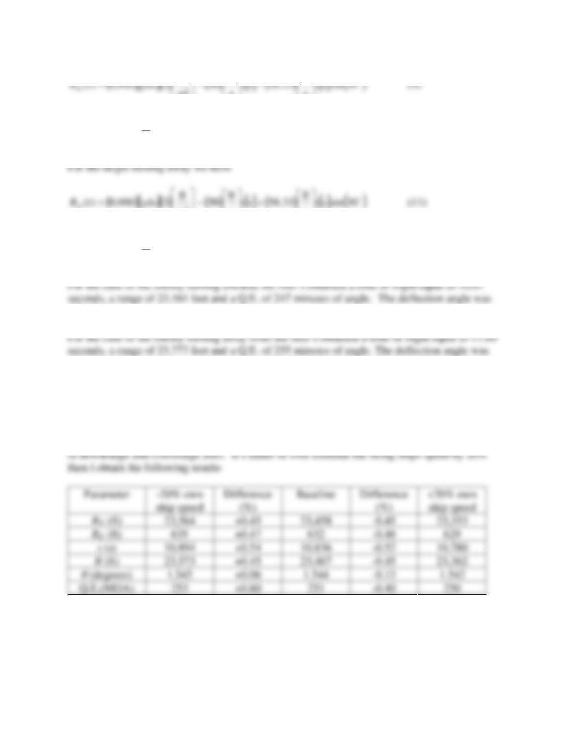
Parameter
-16.7%
target
course
Difference
(%)
Baseline
Difference
(%)
+16.7%
target
course
RN (ft)
23,155
-1.29
23,458
+1.32
23,771
RE (ft)
539
-14.7
632
-0.48
556
t (s)
10.670
-1.53
10.836
+1.52
11.003
R (ft)
23,161
-1.30
23,467
+1.30
23,777
θ (degrees)
1.334
-14.2
1.544
-13.2
1.340
Q.E.(MOA)
247
-1.59
251
+1.57
255
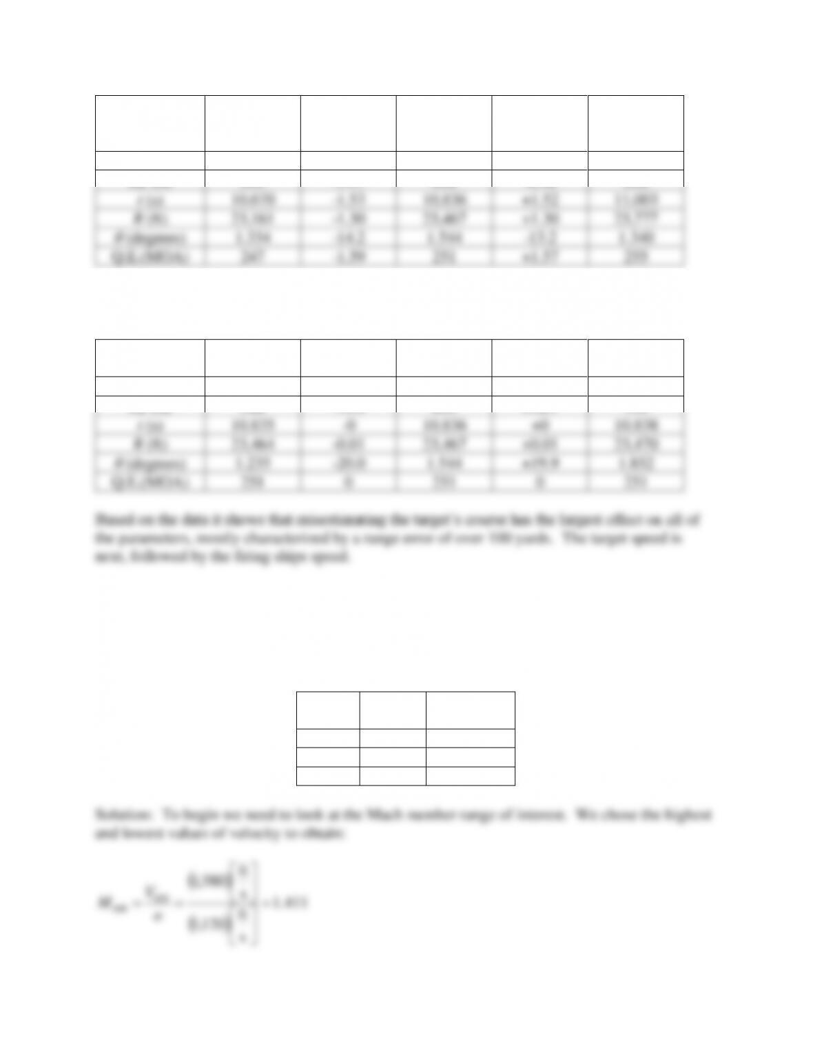
For an incorrect target speed we can use the results of part a.) of the problem again as a basis for
comparison. The results are as follows
Parameter
-20% target
ship speed
Difference
(%)
Baseline
Difference
(%)
+20% target
ship speed
RN (ft)
23,458
0
23,458
0
23,458
RE (ft)
506
-19.9
632
+16.7
759
t (s)
10.835
-0
10.836
+0
10.838
R (ft)
23,464
-0.01
23,467
+0.01
23,470
θ (degrees)
1.235
-20.0
1.544
+19.9
1.852
Q.E.(MOA)
251
0
251
0
251
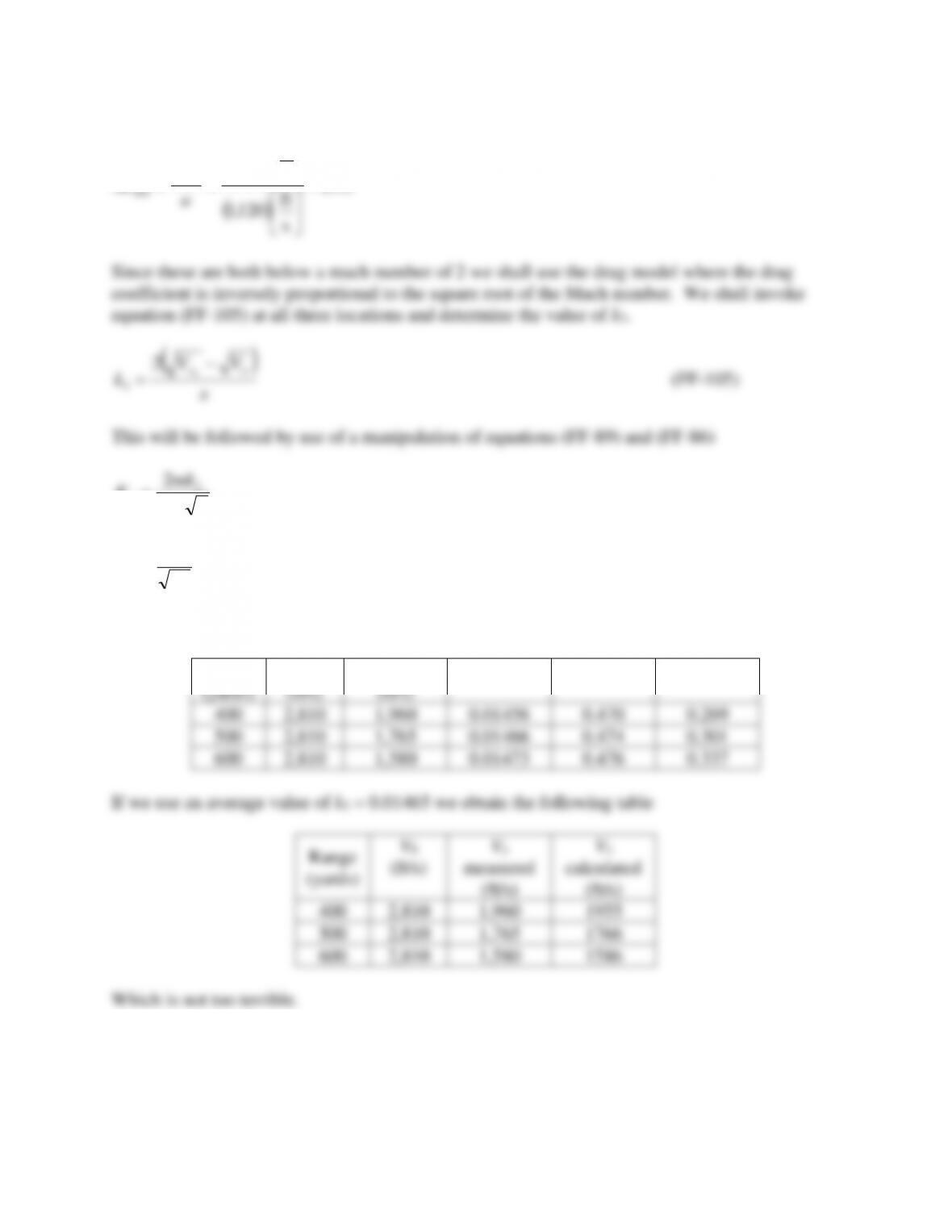
Problem 20 – The U.S. 7.62 mm Ball M80 (projectile diameter = 0.308”, mass m = 147 grains)
is fired in a test range. Based on data below, estimate the coefficient CD. Assume the projectile
is fired with a muzzle velocity of 2,810 ft/s, under standard sea level met conditions (
= 0.0751
lbm/ft3, a = 1120 ft/s). Justify your and answer by explaining why you chose the appropriate
drag model. Validate your answer with an appropriate calculation.
Range
(yards)
V0
(ft/s)
Vx
(ft/s)
400
2,810
1,960
500
2,810
1,765
600
2,810
1,580
( )
s
ft
120,1
600 =
( )
( )
75.1
s
ft
120,1
s
ft
960,1
400
400 =
== a
V
M
aS
mk
K
23
3
=
M
K
CD
3
=
(FF-86)
So our values are
Range
(yards)
V0
(ft/s)
Vx
(ft/s)
k3
K3
CD
400
2,810
1,960
0.01456
0.470
0.269
500
2,810
1,765
0.01466
0.474
0.301
600
2,810
1,580
0.01473
0.476
0.337
If we use an average value of k3 = 0.01465 we obtain the following table
Range
(yards)
V0
(ft/s)
Vx
measured
(ft/s)
Vx
calculated
(ft/s)
400
2,810
1,960
1955
500
2,810
1,765
1766
600
2,810
1,580
1586
Which is not too terrible.
Problem 21 – Many times all of the data we need for a projectile is not provided to us and we
have to extract the information from different sources. You are given the following information
about a British 2 pounder projectile [3]:
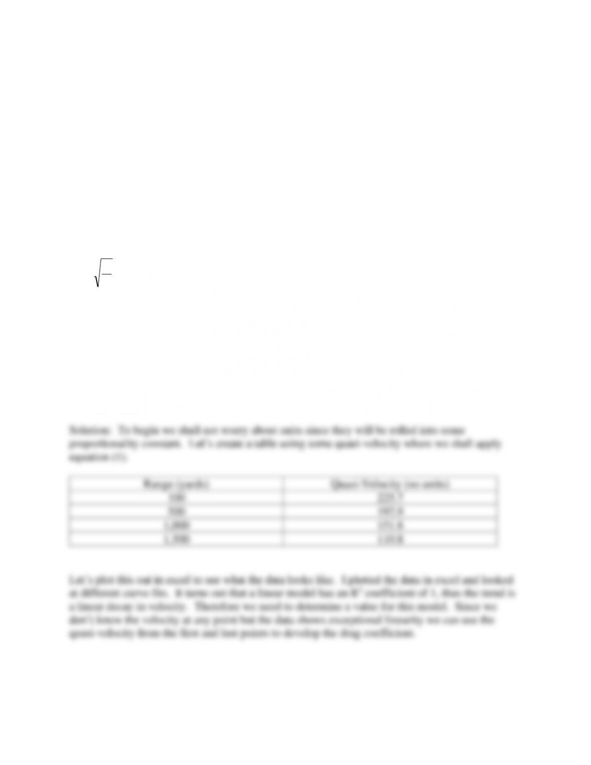
Projectile diameter: 40 mm
Projectile weight: 2.375 lbm
Muzzle velocity: 2,600 ft/s
Armor penetration as a function of distance
Distance (yards) Thickness perforated (mm)
100 55
500 47
1,000 37
1,500 27
In terminal ballistics we will find that, based on some work by Zener and Holloman in 1942 the
penetration of this type of projectile is proportional to the velocity as follows
m
d
tV ~
(1)
Here t is the target thickness, d is the projectile diameter and m is the projectile mass. With only
this information at your disposal:
a.) Determine the best drag model for this projectile
b.) Generate the proper coefficient from the data
c.) Create a table of range (yards), velocity (ft/s), time of flight (s), launch angle
(minutes), impact angle (minutes) if the projectile is fired with no wind at each
position.
Please justify your answer.
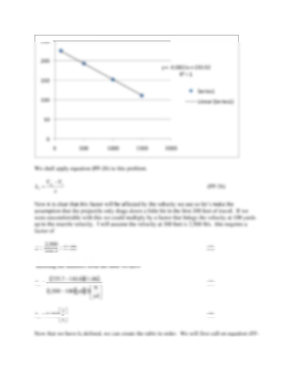
y = -0.0821x + 233.92
R² = 1
0
50
100
150
200
250
0500 1000 1500 2000
Series1
Linear (Series1)
xkVV xx 2
0−=
(FF-73)
Now that we have the impact velocity we can obtain the time of flight from equation (5.68)
0
0
01
ln
x
x
x
x
x
V
V
V
V
V
x
t
−
=
(FF-77)
The elevation angle of the weapon is determined by solving equation (FF-85) for
0 with y and y0
set equal to zero. Thus we have
−
−
=
x
x
x
x
x
x
V
V
V
V
V
V
x
gt
0
0
0ln
1
1
ln
2
2
1
tan
2
0
(5)
For the final task we calculate the angle of fall from equation (FF-80) below
−
−=
x
x
x
x
x
V
V
V
V
V
gt
0
0
0ln
1
tantan 0
(FF-80)
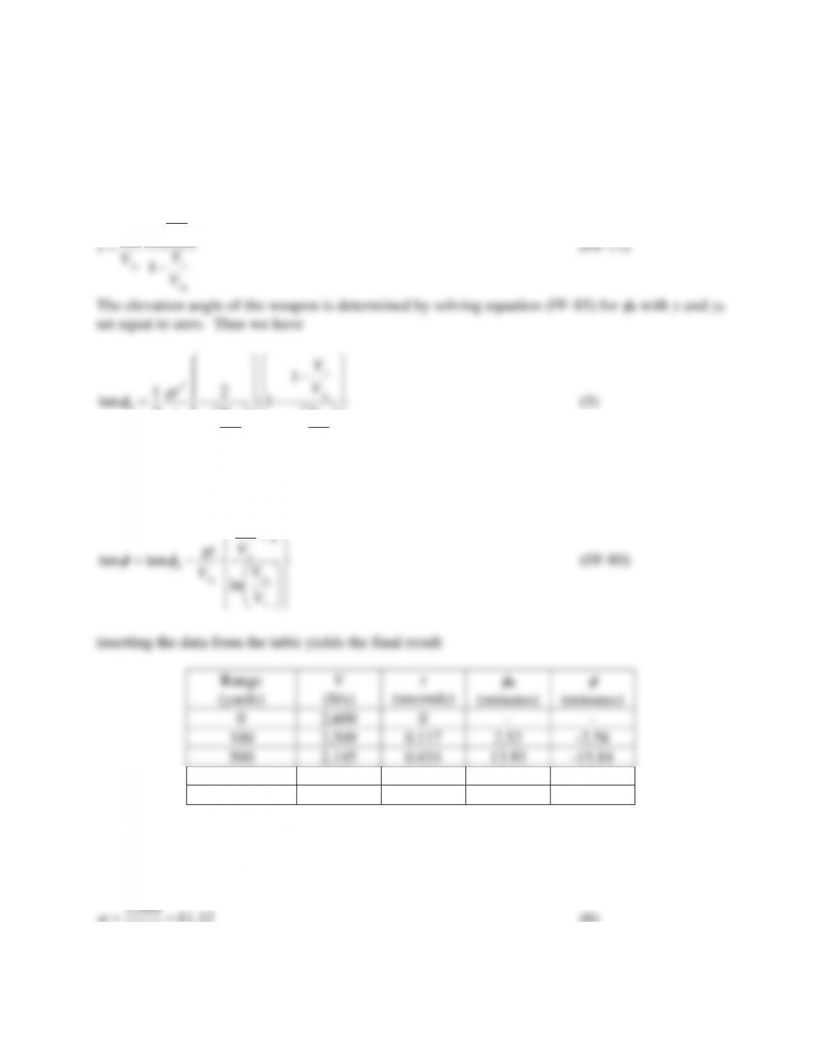
inserting the data from the table yields the final result
Range
(yards)
V
(ft/s)
t
(seconds)
0
(minutes)
(minutes)
0
2,600
0
–
–
100
2,509
0.117
2.52
-2.58
500
2,145
0.634
13.93
-15.84
1,000
1,691
1.420
32.38
-45.15
1,500
1,236
2.453
58.62
-96.30
Notice in this table that we had assumed the velocity came down to 2,500 ft/s in the first 100
yards and the results showed 2,509 ft/s using the k2 value we came up with. We now can iterate
using the new value. If we perform the same calculations but now use
12.11
7.225
509,2 ==a
(6)

[4] Litz, Bryan, Applied Ballistics for Long Range Shooting, 2nd Ed., Applied Ballistics, Cedar
Springs, MI, 2011.
11 22 K
m
m
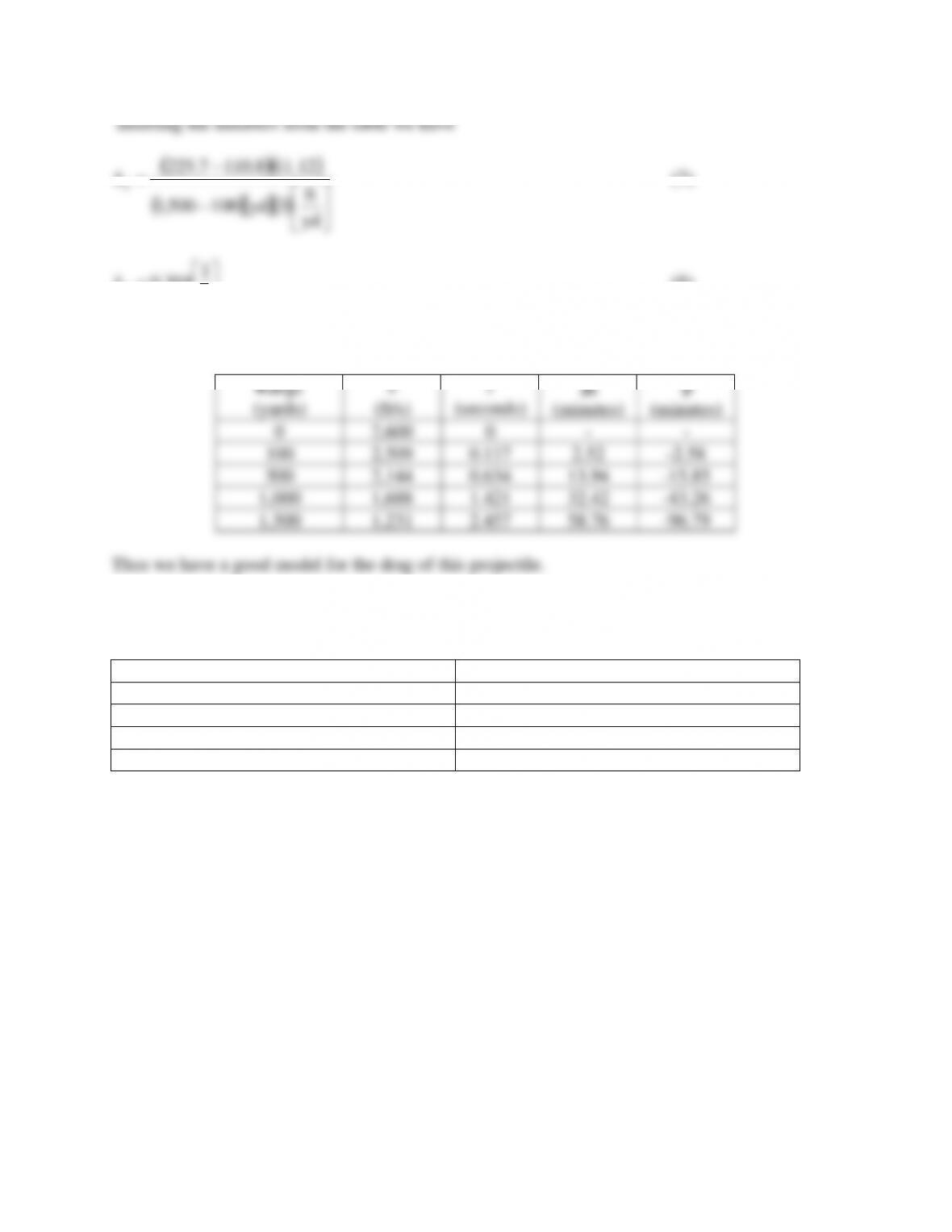
If we make a table of these values we obtain
V [ft/s]
CD
k1[1/m]
1500
0.354
2.315×10⁻⁴
2000
0.306
2.001×10⁻⁴
2500
0.274
1.792×10⁻⁴
3000
0.250
1.635×10⁻⁴
We will have to take an average value for k1 from this table and we obtain
= −
m
1
10935.1 4
1AVG
k
S
mk
CAVG
est
D
1
2
=
and
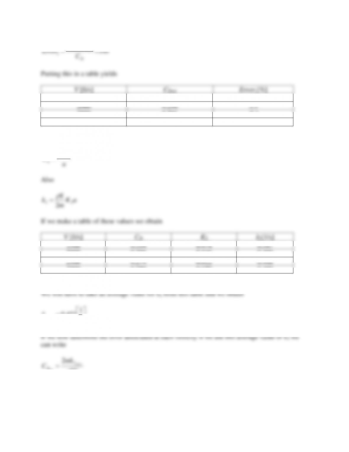
100
1
−
=
D
DD
C
CC
Error est
Putting this in a table yields
V [ft/s]
CDest
Error1[%]
1500
0.296
16
2000
0.296
3.3
2500
0.296
-8.1
3000
0.296
-18.4
Now let’s look at the second model where we see that
a
VC
KD
=
2