Chapter 19: Estimating Default Probabilities
19.23. (Spreadsheet Provided)
Suppose a three-year corporate bond provides a coupon of 7% per year payable semiannually
and has a yield of 5% (expressed with semiannual compounding). The yields for all maturities on
risk-free bonds is 4% per annum (expressed with semiannual compounding). Assume that
defaults can take place every six months (immediately before a coupon payment) and the
recovery rate is 45%. Estimate the default probabilities assuming a) the unconditional default
probabilities are the same on each possible default date and b) assuming that the default
probabilities conditional on no earlier default are the same on each possible default date.
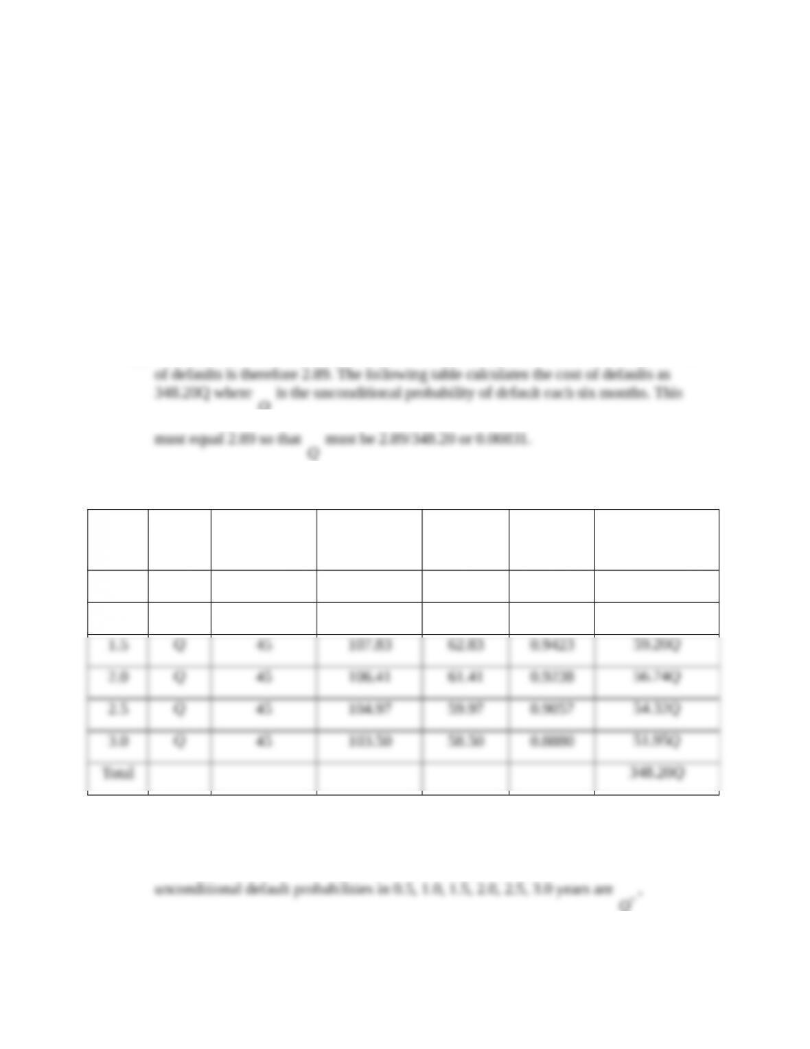
(a) The market price of the bond is 105.51. The risk-free price is 108.40. The expected cost
Q
Q
Time
(yrs)
Def.
Prob.
Recovery
Amount ($)
Risk-free
Value ($)
Loss
Given
Default ($)
Discount
Factor
PV of Expected
Loss ($)
0.5
Q
45 110.57 65.57 0.9804
64 28Q.
1.0
Q
45 109.21 64.21 0.9612
61 73Q.
Q
59 20Q.

(1 )Q Q
* *
–
,
2
(1 )Q Q
* *
–
,
3
(1 )Q Q
* *
–
,
4
(1 )Q Q
* *
–
,
5
(1 )Q Q
* *
–
. We must therefore find
the value of
Q
*
that solves
2 3
64 28 61 73 (1 ) 59 20 (1 ) 56 74 (1 )Q Q Q Q Q Q Q
* * * * * * *
. + . – + . * – + . –
4 5
54 32 (1 ) 51 95 (1 ) 2 89Q Q Q Q
* * * *
+ . – + . – = .
Using Solver in Excel we find that
0 00848Q
*
= .
.
19.24.
A company has one- and two-year bonds outstanding, each providing a coupon of 8% per year
payable annually. The yields on the bonds (expressed with continuous compounding are 6.0%
and 6.6%, respectively. Risk-free rates are 4.5% for all maturities. The recovery rate is 35%.
Defaults can take place half way through each year. Estimate the risk-neutral default rate each
year.
Consider the first bond. Its market price is
0 06 1
108 101 71e
– . ´
= .
. Its default-free price is
0 045 1
108 103 25e
– . ´
= .
. The present value of the loss from defaults is therefore 1.54. In this case
losses can take place at only one time, halfway through the year. Suppose that the probability of
default at this time is
1
Q
. The default-free value of the bond is
0 045 0 5
108 105 60e
– . ´ .
= .
. The loss in
the event of a default is
105 60 35 70 60. – = .
. The present value of the expected loss is
0 045 0 5
1 1
70 60 69 03e Q Q
– . ´ .
. = .
. It follows that
1
69 03 1 54Q. = .
so that
10 0223Q= .
.
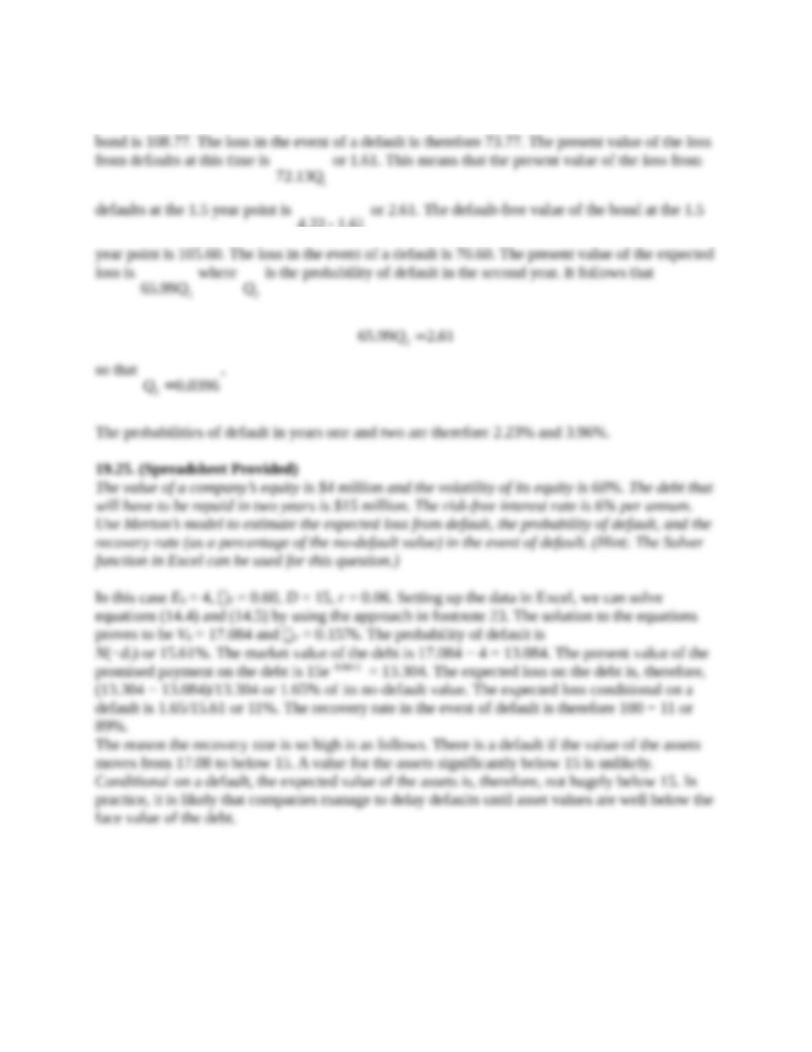
Now consider the second bond. It market price is 102.13 and its default-free value is 106.35. The
present value of the loss from defaults is therefore 4.22. At time 0.5 the default free value of the
2
65 99Q.
2
Q
2
65 99 2 61Q. = .
so that
2
0 0396Q= .
.
19.25. (Spreadsheet Provided)
The value of a company’s equity is $4 million and the volatility of its equity is 60%. The debt that
will have to be repaid in two years is $15 million. The risk-free interest rate is 6% per annum.
Use Merton’s model to estimate the expected loss from default, the probability of default, and the
recovery rate (as a percentage of the no-default value) in the event of default. (Hint: The Solver
function in Excel can be used for this question.)
In this case E0 = 4, E = 0.60, D = 15, r = 0.06. Setting up the data in Excel, we can solve
equations (14.4) and (14.5) by using the approach in footnote 23. The solution to the equations
The reason the recovery rate is so high is as follows. There is a default if the value of the assets
moves from 17.08 to below 15. A value for the assets significantly below 15 is unlikely.