Chapter 14: Model-Building Approach
14.16.
Consider a position consisting of a $300,000 investment in gold and a $500,000 investment in
silver. Suppose that the daily volatilities of these two assets are 1.8% and 1.2% respectively, and
that the coefficient of correlation between their returns is 0.6. What is the 10-day 97.5% VaR for
the portfolio? By how much does diversification reduce the VaR?
The variance of the portfolio (in thousands of dollars) is
The standard deviation is
04.104
= 10.2. Since N(−1.96) = 0.025, the 1-day 97.5% VaR is 10.2
10
14.17.
Consider a portfolio of options on a single asset. Suppose that the delta of the portfolio is 12, the
value of the asset is $10, and the daily volatility of the asset is 2%. Estimate the one-day 95%
VaR for the portfolio from the delta.
An approximate relationship between the daily change in the value of the portfolio, P and the
proportional daily change in the value of the asset x is
The standard deviation of x is 0.02. It follows that the standard deviation of P is 2.4. The 1
14.18.
Suppose that you know the gamma of the portfolio in Problem 15.17 is –2.6. Derive a quadratic
relationship between the change in the portfolio value and the percentage change in the
underlying asset price in one day.
(a) Calculate the first three moments of the change in the portfolio value.
(b) Using the first two moments and assuming that the change in the portfolio is normally
distributed, calculate the one-day 95% VaR for the portfolio.
(c) Use the third moment and the Cornish–Fisher expansion to revise your answer to (b).
Using the same notation as in Problem 15.17, the quadratic relationship is
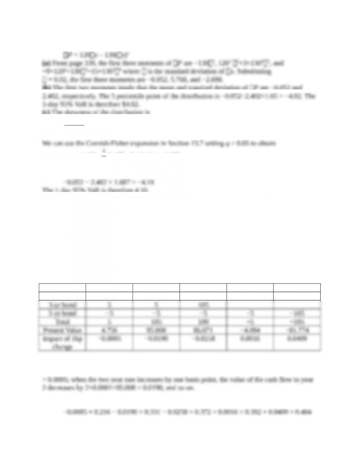
or
(b) The first two moments imply that the mean and standard deviation of P are −0.052 and
(c) The skewness of the distribution is
13.0052.02052.0768.53698.2
402.2
1
2
3
.
Assuming one factor, the standard deviation of the one-day change in the portfolio value is
20
Assuming two factors, the standard deviation of the one-day change in the portfolio value is
0785.077.401589.055.1700116.0
2222
20
Assuming three factors, the standard deviation of the one-day change in the portfolio value is
610.008.201283.077.401589.055.1700116.0
222222
20
In this case the second has the most important impact on VaR.
14.20.
A company has a position in bonds worth $6 million. The modified duration of the portfolio is
5.2 years. Assume that only parallel shifts in the yield curve can take place and that the standard
deviation of the daily yield change (when yield is measured in percent) is 0.09. Use the duration
model to estimate the 20-day 90% VaR for the portfolio. Explain carefully the weaknesses of this
approach to calculating VaR. Explain two alternatives that give more accuracy.
The change in the value of the portfolio for a small change y in the yield is approximately
−DBy where D is the duration and B is the value of the portfolio. It follows that the standard
deviation of the daily change in the value of the bond portfolio equals DBy where y is the
20
approach assumes that only parallel shifts in the term structure can take place. Equivalently it
14.21. (Spreadsheet Provided)
A bank has written European a call option on one stock and a European put option on another
stock. For the first option, the stock price is 50, the strike price is 51, the volatility is 28% per
annum, and the time to maturity is nine months. For the second option, the stock price is 20, the
strike price is 19, the volatility is 25% per annum, and the time to maturity is one year. Neither
stock pays a dividend, the risk-free rate is 6% per annum, and the correlation between stock
price returns is 0.4. Calculate a 10-day 99% VaR
(a) Using only deltas.
(b) Using the partial simulation approach.
(c) Using the full simulation approach.
This assignment is useful for consolidating students’ understanding of alternative approaches to
calculating VaR, but it is calculation intensive. Students should have some Excel (ideally VBA)
10
calculate a 10-day VaR directly, which is fine.)
(a) From DerivaGem, the values of the two option positions are –5.413 and –1.014.
or
25228.0
25225.0
respectively. The one-day variance of P is
The one day standard deviation is, therefore, 0.4906 and the 10-day 99% VaR is
10
(b) In the partial simulation approach, we simulate changes in the stock prices over a one-day
period (building in the correlation) and then use the quadratic approximation to calculate the
(c) In the full simulation approach, we simulate changes in the stock price over one day (building
14.22.
A common complaint of risk managers is that the model-building approach (either linear or
quadratic) does not work well when delta is close to zero. Test what happens when delta is close
to zero in using Sample Application E in the DerivaGem Application Builder software. (You can
do this by experimenting with different option positions and adjusting the position in the
underlying to give a delta of zero.) Explain the results you get.
We can create a portfolio with zero delta in Sample Application E by changing the position in the
Other zero-delta examples can be created by changing the option portfolio and then zeroing out
delta by adjusting the position in the underlying asset. The results are similar. The software
shows that neither the linear model nor the quadratic model gives good answers when delta is
14.23. (Spreadsheet Provided)
The calculations in Section 15.3 assume that the investments in the DJIA, FTSE 100, CAC 40,
and Nikkei 225 are $4 million, $3 million, $1 million, and $2 million, respectively. How do the
VaR and ES change if the investment are $3million, $3 million, $1 million, and $3 million,
respectively? Carry out calculations when (a) volatilities and correlations are estimated
using the equally weighted model and (b) when they are estimated using the EWMA model. What
is the effect of changing from 0.94 to 0.90 in the EWMA calculations? Use the spreadsheets on
the author’s web site.
(a) When the equally weighted model is used the worksheet shows that one-day 99% VaR is
(b) When the EWMA model is used the worksheet shows that one-day 99% VaR is $447,404.