Chapter 13: The Historical Simulation and Extreme Value Theory
13.12.
Suppose that a one-day 97.5% VaR is estimated as $13 million from 2,000 observations. The
one-day changes are approximately normal with mean zero and standard deviation $6 million.
Estimate a 99% confidence interval for the VaR estimate.
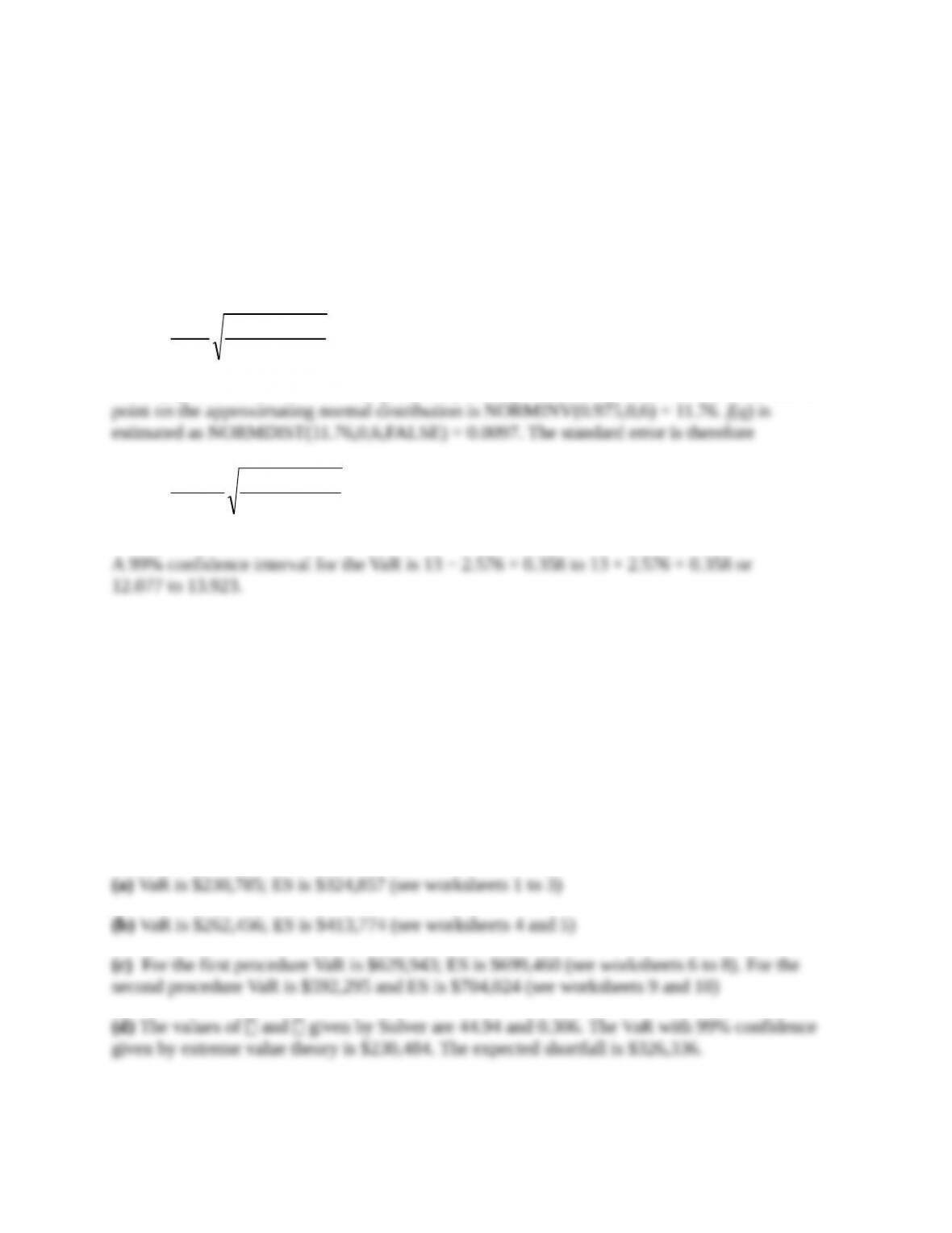
The standard error is
2000
975.0025.0
)(
1
qf
where f(q) is an estimate of the loss probability density at the VaR point. In this case the 0.975
point on the approximating normal distribution is NORMINV(0.975,0,6) = 11.76. f(q) is
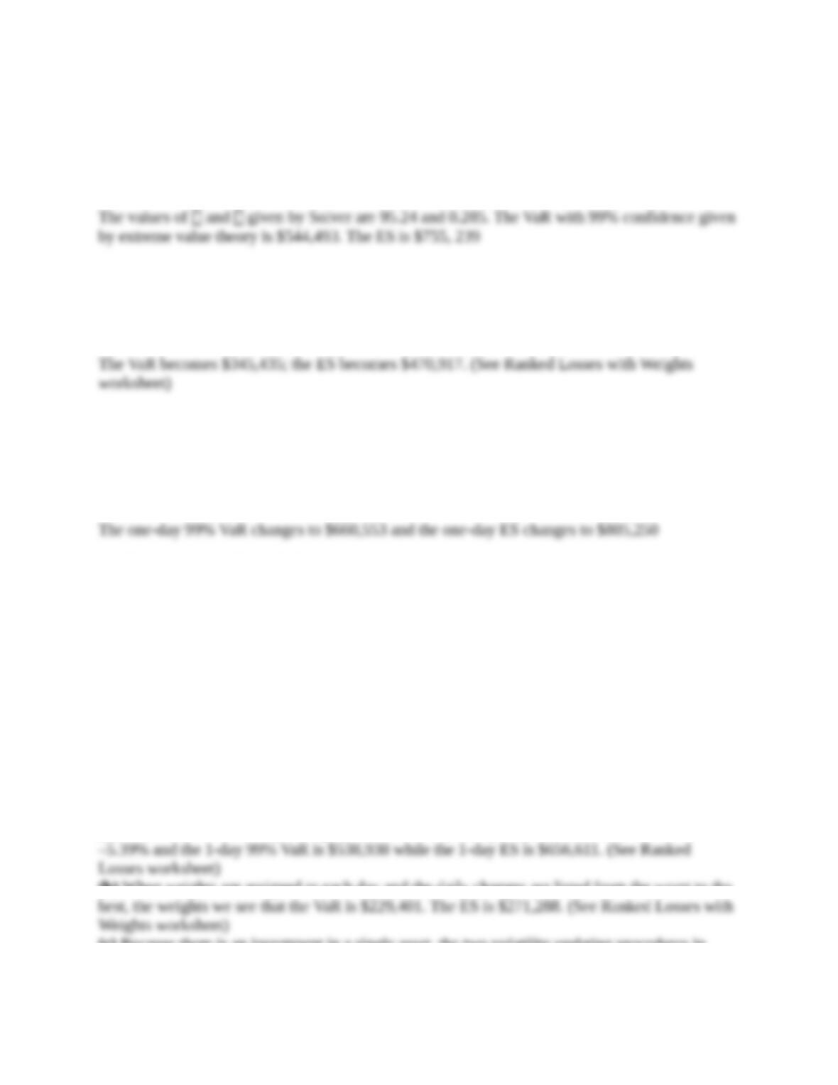
estimated as NORMDIST(11.76,0,6,FALSE) = 0.0097. The standard error is therefore
358.0
2000
975.0025.0
0097.0
1
A 99% confidence interval for the VaR is 13 − 2.576 × 0.358 to 13 + 2.576 × 0.358 or
12.077 to 13.923.
13.13. (Spreadsheet Provided)
Suppose that the portfolio considered in Section 13.1 has (in $000s) 3,000 in DJIA, 3,000 in
FTSE, 1,000 in CAC 40, and 3,000 in Nikkei 225. Use the spreadsheet on the author’s web site to
calculate what difference this makes to
(a) The one-day 99% VaR and ES that are calculated in Section 13.1.
(b) The one-day 99% VaR and ES that are calculated using the weighting-of observations
procedure in Section 13.3 and=0.995
(c) The one-day 99% VaR and ES that are calculated using the two volatility-updating
procedures in Section 13.3 and = 0.94. (Assume that the initial variance when EWMA is
applied is the sample variance.)
(d) The one-day 99% VaR and ES that are calculated using extreme value theory in Section 13.6.
13.14. (Spreadsheet Provided)
Investigate the effect of applying extreme value theory to the volatility adjusted results in Section
13.3 with u = 350.
13.15. (Spreadsheet Provided)
The “weighting-of-observations” procedure in Section 13.3 gives the one-day 99% VaR equal to
$282,204 and the one-day ES as $400,583. Use the spreadsheets on the author’s web site to
calculate these measures when the parameter in this procedure is changed from 0.995 to 0.99.
13.16. (Spreadsheet Provided)
The first “volatility-updating” procedure in Section 13.3 gives the one-day 99% VaR equal to
$602,968 and the one-day 99% ES equal to $750,078. Use the spreadsheets on the author’s web
site to calculate the VaR and ES when the parameter in this procedure is changed from 0.94 to
0.92.
13.17 (Spreadsheet Provided)
Values for the NASDAQ composite index during the 1,500 days preceding March 10, 2006, can
be downloaded from the author’s web site. Calculate the one-day 99% VaR and the one-day 99%
ES on March 10, 2006, for a $10 million portfolio invested in the index using
(a) The basic historical simulation approach.
(b) The exponential weighting scheme in Section 13.3 with = 0.995.
(c) The volatility-updating procedures in Section 13.3 with = 0.94. (Assume that the initial
variance when EWMA is applied is the sample variance.)
(d) Extreme value theory with u = 300 and equal weightings.
(e) A model where daily returns are assumed to be normally distributed with mean zero. (Use
both an equally weighted approach and the EWMA approach with = 0.94 to estimate the
standard deviation of daily returns.)
Discuss the reasons for the differences between the results you get.
(a) The fifteenth worst daily change in the NASDAQ during the period considered is about
(b) When weights are assigned to each day and the daily changes are listed from the worst to the
(c) Because there is an investment in a single asset, the two volatility updating procedures in
Section 13.3 are equivalent. We can use the EWMA updating scheme to update the variance and
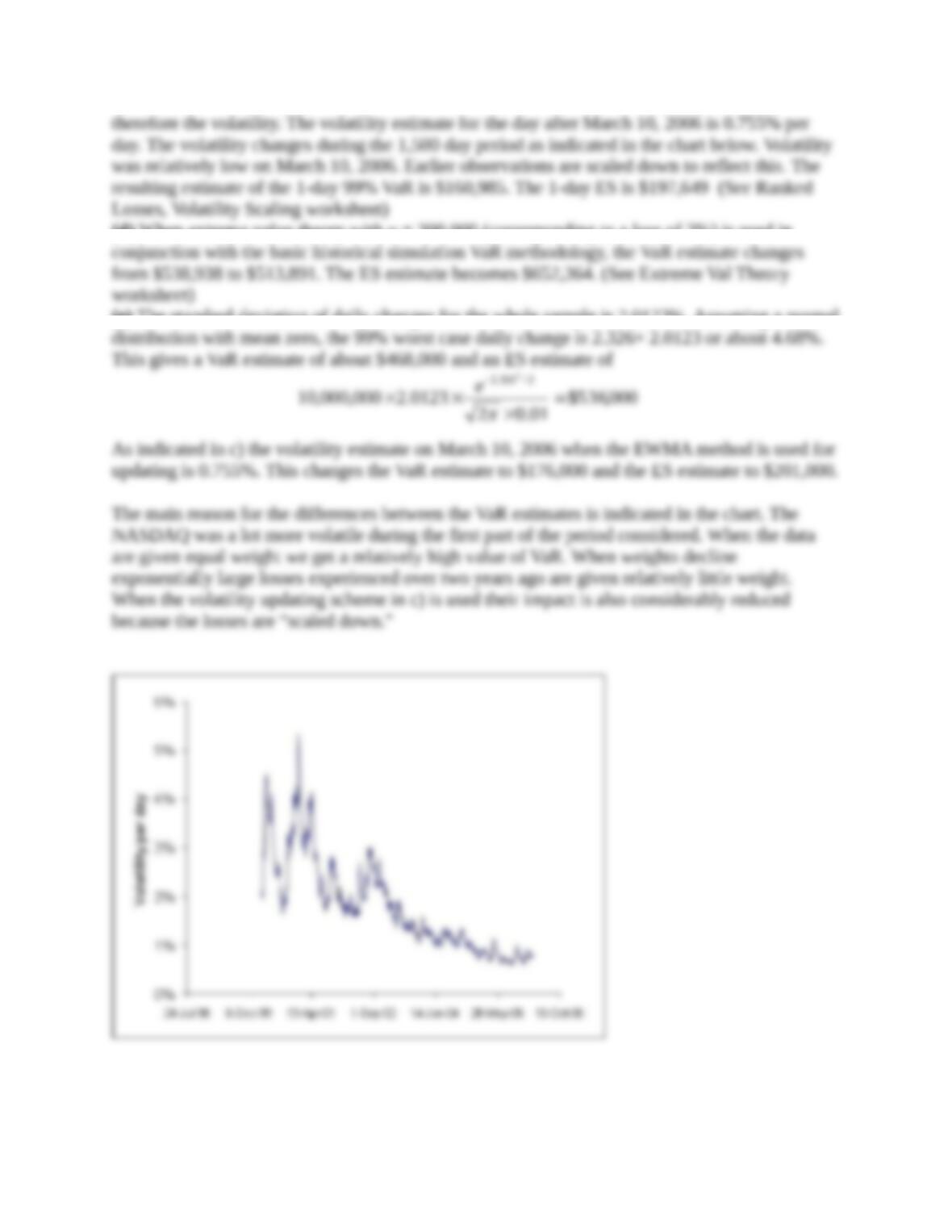
(d) When extreme value theory with u = 300,000 (corresponding to a loss of 3%) is used in
(e) The standard deviation of daily changes for the whole sample is 2.0123%. Assuming a normal