Chapter 11: Correlations and Copulas
11.16.
Suppose that the price of Asset X at close of trading yesterday was $300 and its volatility was
estimated as 1.3% per day. The price of X at the close of trading today is $298. Suppose further
that the price of Asset Y at the close of trading yesterday was $8, its volatility was estimated as
1.5% per day, and its correlation with X was estimated as 0.8. The price of Y at the close
of trading today is unchanged at $8. Update the volatility of X and Y and the correlation between
X and Y using
(a) The EWMA model with = 0.94
(b) The GARCH(1,1) model with = 0.000002, = 0.04, and = 0.94.
In practice, is the parameter likely to be the same for X and Y?
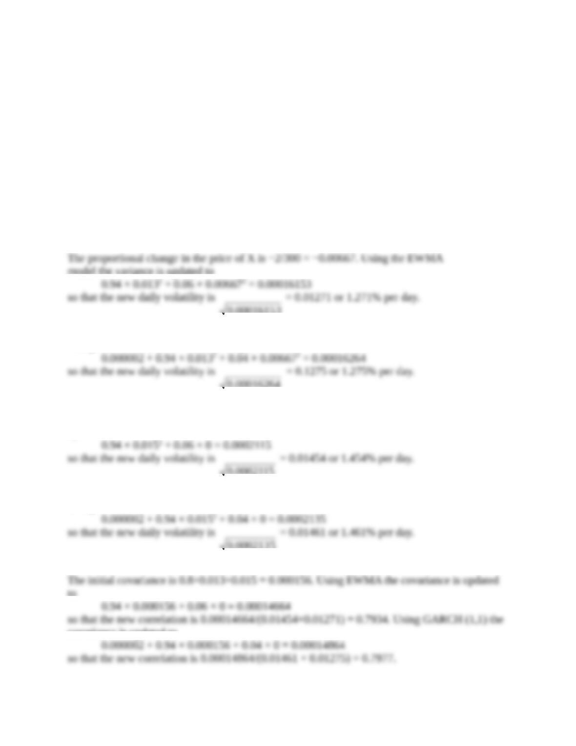
model the variance is updated to
so that the new daily volatility is
00016153.0
= 0.01271 or 1.271% per day.
Using GARCH (1,1), the variance is updated to
00016264.0
The proportional change in the price of Y is zero. Using the EWMA model the variance is
updated to
0002115.0
Using GARCH (1,1), the variance is updated to
so that the new daily volatility is
0002135.0
= 0.01461 or 1.461% per day.
The initial covariance is 0.8×0.013×0.015 = 0.000156. Using EWMA the covariance is updated
to
covariance is updated to
For a given and , the parameter defines the long run average value of a variance or a
covariance. There is no reason why we should expect the long run average daily variance for X
11.17. (Spreadsheet Provided)
The probability density function for an exponential distribution is e−x where x is the value of
the variable and is a parameter. The cumulative probability distribution is 1− e−x. Suppose
that two variables V1 and V2 have exponential distributions with parameters of 1.0 and 2.0,
respectively. Use a Gaussian copula to define the correlation structure between V1 and V2 with a
copula correlation of –0.2. Produce a table similar to Table 11.3 using values of 0.25, 0.5, 0.75,
1, 1.25, and 1.5 for V1 and V2. A spreadsheet for calculating the cumulative bivariate normal
distribution is on the author’s website: www-2.rotman.utoronto.ca/∼hul/riskman.
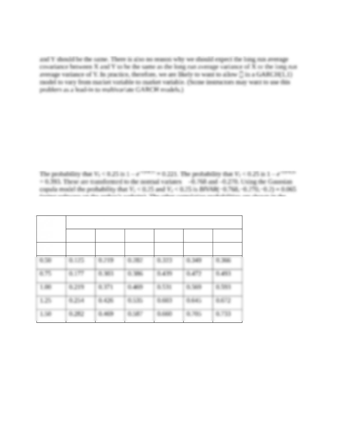
(using software on the author’s website). The other cumulative probabilities are shown in the
table below and are calculated similarly.
V1
V2
0.25 0.50 0.75 1.00 1.25 1.50
0.25 0.065 0.117 0.153 0.177 0.193 0.203
11.18. (Spreadsheet Provided)
Create an Excel spreadsheet to produce a chart similar to Figure 11.5 showing samples from a
bivariate Student’s t-distribution with four degrees of freedom where the correlation is 0.5. Next
suppose that the marginal distributions of V1 and V2 are Student’s t with four degrees of freedom
but that a Gaussian copula with a copula correlation parameter of 0.5 is used to define the
correlation between the two variables. Construct a chart showing samples from the joint
distribution. Compare the two charts you have produced.
The procedure for taking a random sample from a bivariate Student’s t-distribution is described
on page 244. This can be used to produce Figure 11.5. For the second part of the question we
sample U1 and U2 from a bivariate normal distribution where the correlation is 0.5 as described in
11.19. (Spreadsheet Provided)
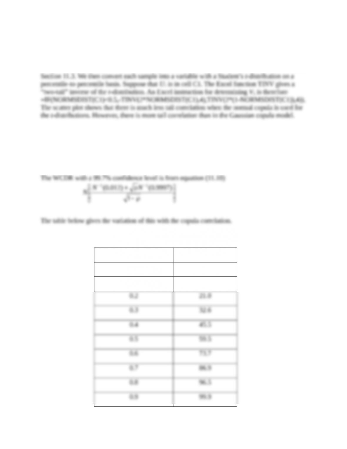
Suppose that a bank has made a large number loans of a certain type. The one-year probability
of default on each loan is 1.2%. The bank uses a Gaussian copula for time to default. It is
interested in estimating a “99.97% worst case” for the percent of loan that default on the
portfolio. Show how this varies with the copula correlation.
11.20. (Spreadsheet Provided)
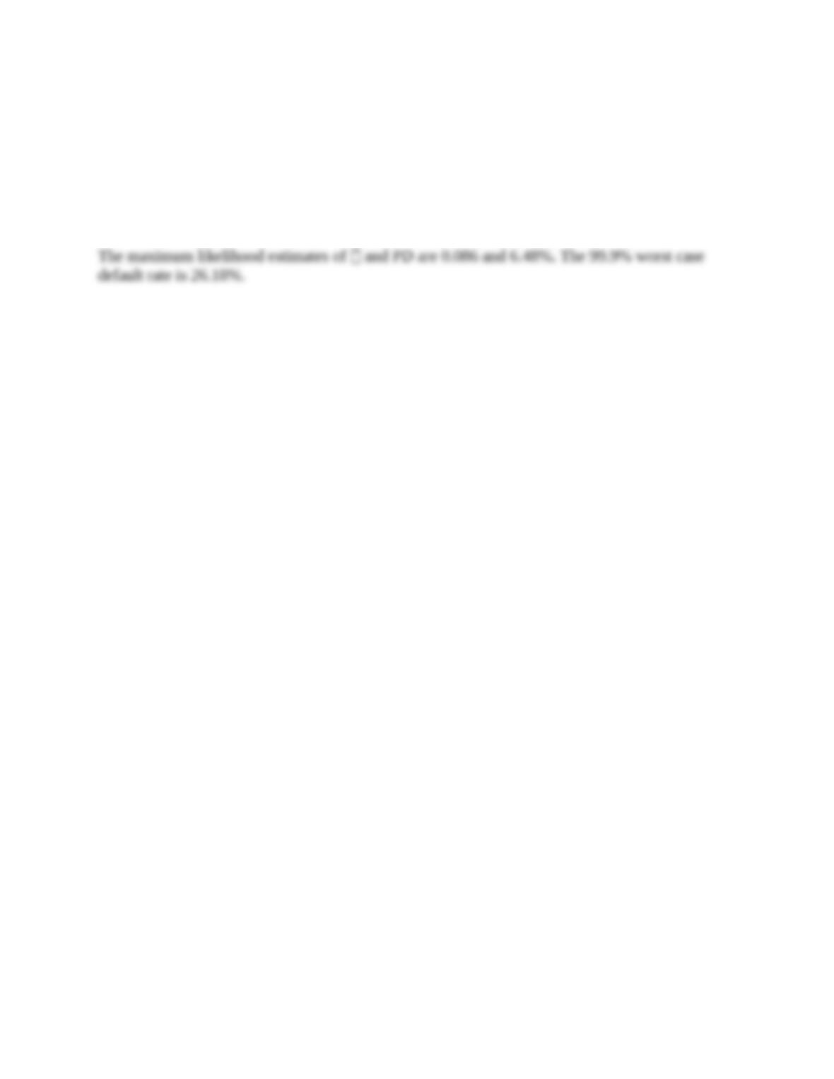
The default rates in the last 15 years for a certain category of loans is 2%, 4%, 7%, 12%, 6%,
5%, 8%, 14%, 10%, 2%, 3%, 2%, 6%, 7%, 9%. Use the maximum likelihood method to calculate
the best fit values of the parameters in Vasicek’s model. What is the probability distribution of
the default rate? What is the 99.9% worst case default rate?