Chapter 10: Volatility
10.18. (Spreadsheet Provided)
Suppose that observations on a stock price (in dollars) at the end of each of 15 consecutive days
are as follows:
30.2, 32.0, 31.1, 30.1, 30.2, 30.3, 30.6, 30.9, 30.5, 31.1, 31.3, 30.8, 30.3, 29.9, 29.8
Estimate the daily volatility using both approaches in Section 10.5?
10.19.
Suppose that the price of an asset at close of trading yesterday was $300 and its volatility was
estimated as 1.3% per day. The price at the close of trading today is $298. Update the volatility
estimate using
(a) The EWMA model with = 0.94
(b) The GARCH(1,1) model with = 0.000002, = 0.04, and = 0.94.
The proportional change in the price of the asset is −2/300 = −0.00667.
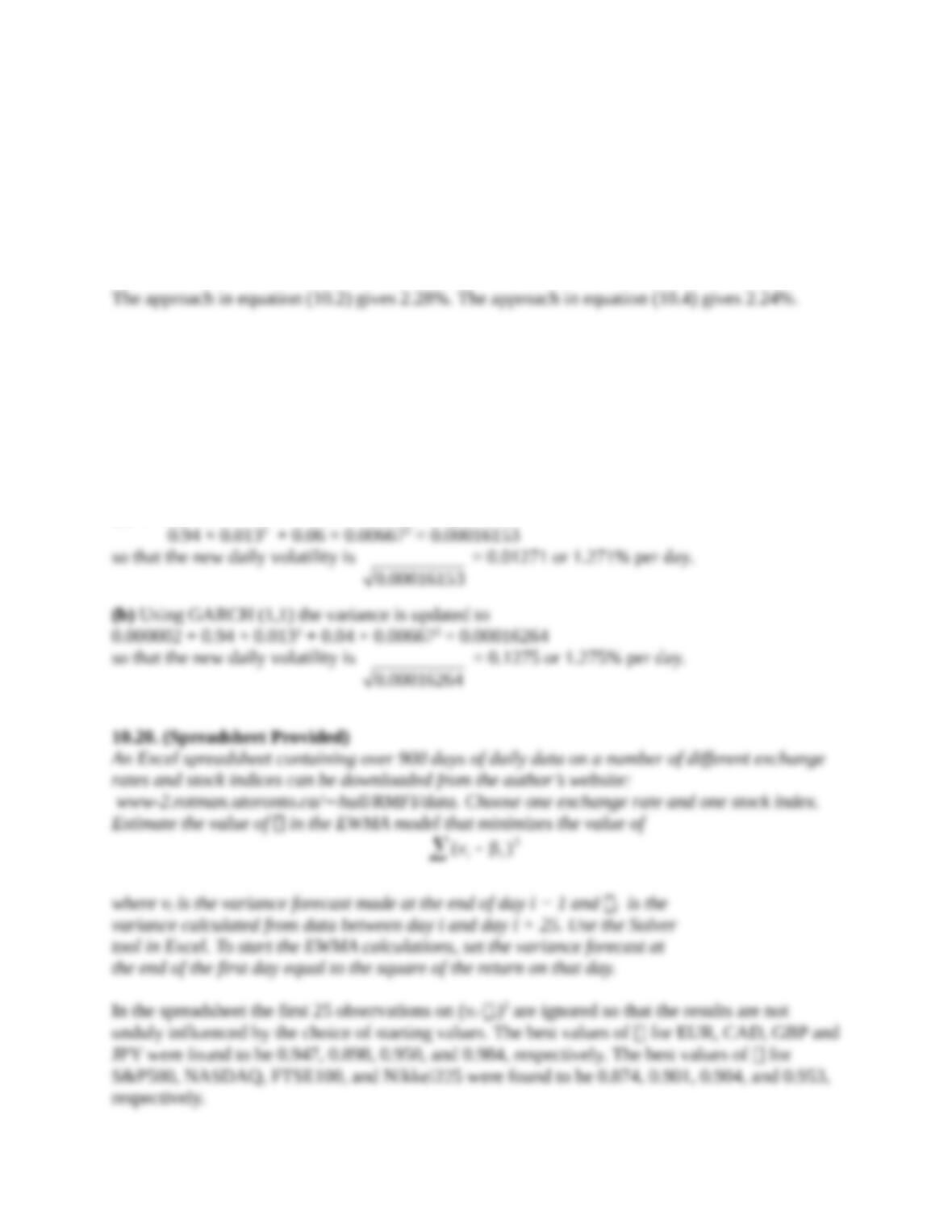
(a) Using the EWMA model the variance is updated to
so that the new daily volatility is
00016153.0
= 0.01271 or 1.271% per day.
(b) Using GARCH (1,1) the variance is updated to
0.000002 + 0.94 × 0.0132 + 0.04 × 0.006672 = 0.00016264
so that the new daily volatility is
00016264.0
= 0.1275 or 1.275% per day.
10.20. (Spreadsheet Provided)
An Excel spreadsheet containing over 900 days of daily data on a number of different exchange
rates and stock indices can be downloaded from the author’s website:
www-2.rotman.utoronto.ca/∼hull/RMFI/data. Choose one exchange rate and one stock index.
Estimate the value of in the EWMA model that minimizes the value of
2
)(
ii
v
where vi is the variance forecast made at the end of day i − 1 and i is the
variance calculated from data between day i and day i + 25. Use the Solver
tool in Excel. To start the EWMA calculations, set the variance forecast at
the end of the first day equal to the square of the return on that day.
In the spreadsheet the first 25 observations on (vi–i)2 are ignored so that the results are not
unduly influenced by the choice of starting values. The best values of for EUR, CAD, GBP and
10.21.
Suppose that the parameters in a GARCH(1,1) model are = 0.03, = 0.95 and = 0.000002.
(a) What is the long-run average volatility?
(b) If the current volatility is 1.5% per day, what is your estimate of the
volatility in 20, 40, and 60 days?
(c) What volatility should be used to price 20-, 40-, and 60-day options?
(d) Suppose that there is an event that increases the volatility from 1.5% per day to 2% per day.
Estimate the effect on the volatility in 20, 40, and 60 days.
(e) Estimate by how much the event increases the volatilities used to price 20-, 40-, and 60-day
options.
(a) The long-run average variance, VL, is
0001.0
02.0
000002.0
1
The long run average volatility is
0001.0
= 0.01 or 1% per day.
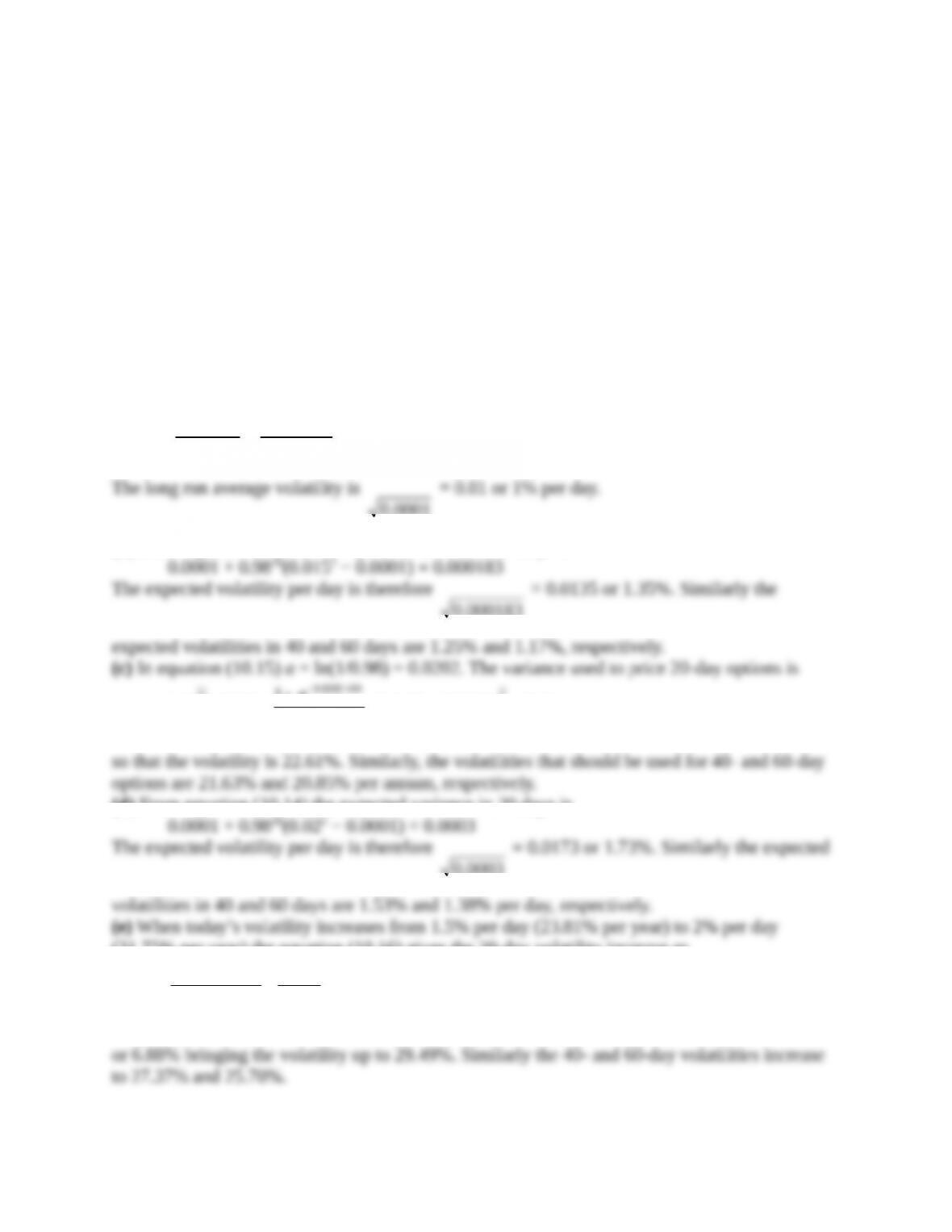
(b) From equation (10.14) the expected variance in 20 days is
The expected volatility per day is therefore
000183.0
= 0.0135 or 1.35%. Similarly the
expected volatilities in 40 and 60 days are 1.25% and 1.17%, respectively.
(c) In equation (10.15) a = ln(1/0.98) = 0.0202. The variance used to price 20-day options is
051.0)0001.0015.0(
200202.0
1
0001.0252
2
200202.0
e
so that the volatility is 22.61%. Similarly, the volatilities that should be used for 40- and 60-day
options are 21.63% and 20.85% per annum, respectively.
(d) From equation (10.14) the expected variance in 20 days is
The expected volatility per day is therefore
0003.0
= 0.0173 or 1.73%. Similarly the expected
volatilities in 40 and 60 days are 1.53% and 1.38% per day, respectively.
(e) When today’s volatility increases from 1.5% per day (23.81% per year) to 2% per day
(31.75% per year) the equation (10.16) gives the 20-day volatility increase as
88.6)81.2375.31(
61.22
81.23
200202.0
1200202.0
e
or 6.88% bringing the volatility up to 29.49%. Similarly the 40- and 60-day volatilities increase
to 27.37% and 25.70%.
10.22. (Spreadsheet Provided)
Estimate parameters for the EWMA and GARCH(1,1) model on the euro-USD exchange rate
data between July 27, 2005, and July 27, 2010. This data can be found on the author’s website:
www-2.rotman.utoronto.ca/∼hull/RMFI/data
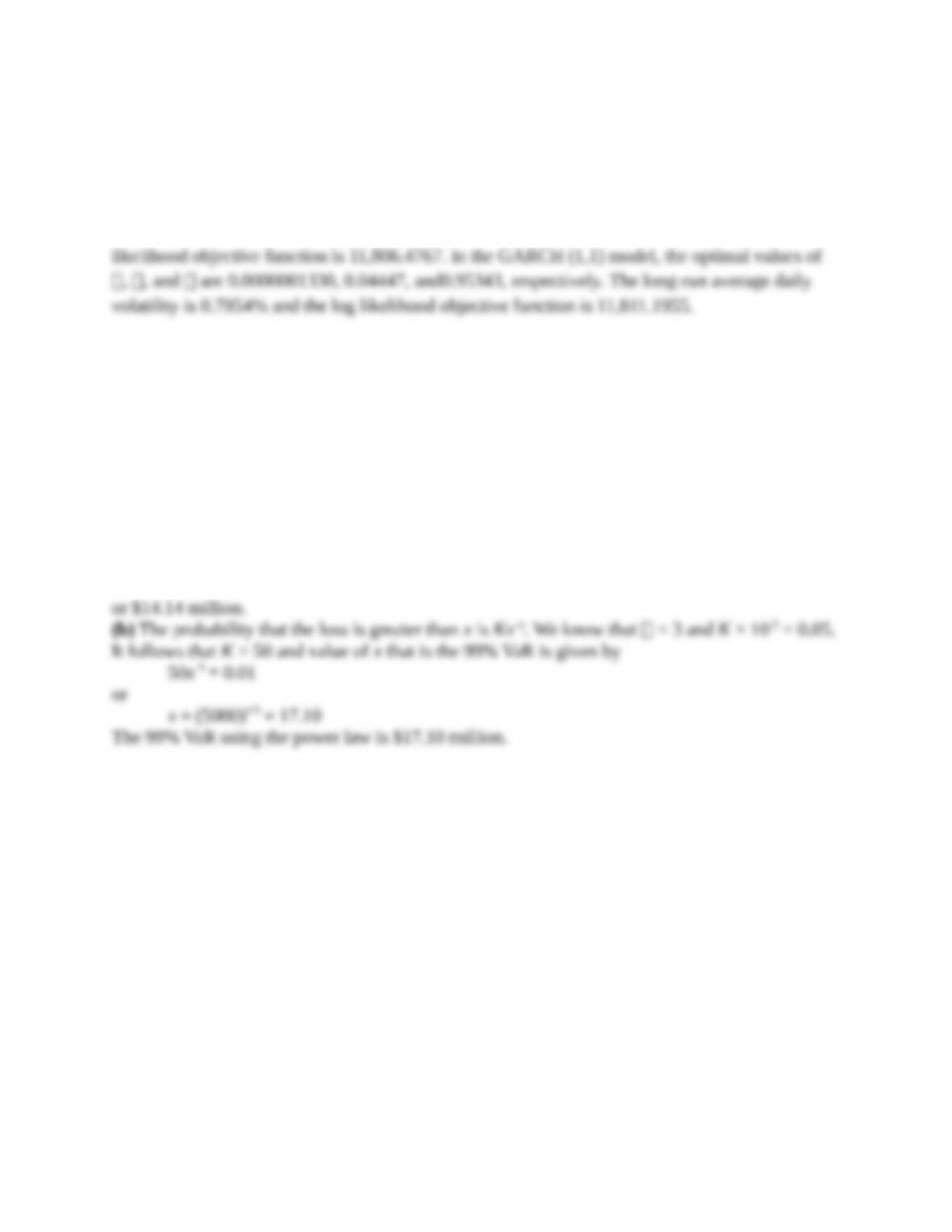
As the spreadsheets show the optimal value of in the EWMA model is 0.958 and the log
10.23.
The probability that the loss from a portfolio will be greater than $10 million in one month is
estimated to be 5%.
(a) What is the one-month 99% VaR assuming the change in value of the portfolio is normally
distributed with zero mean?
(b) What is the one-month 99% VaR assuming that the power law applies with a = 3?
(a) The 99% VaR is
14.14
)95.0(
)99.0(
10 1
1
N
N
or $14.14 million.
(b) The probability that the loss is greater than x is Kx–. We know that = 3 and K × 10-3 = 0.05.
It follows that K = 50 and value of x that is the 99% VaR is given by
50x-3 = 0.01
or
x = (5000)1/3 = 17.10
The 99% VaR using the power law is $17.10 million.