Valuation: Measuring and Managing the Value of Companies, Sixth Edition
Chapter 35 Flexibility
Solutions
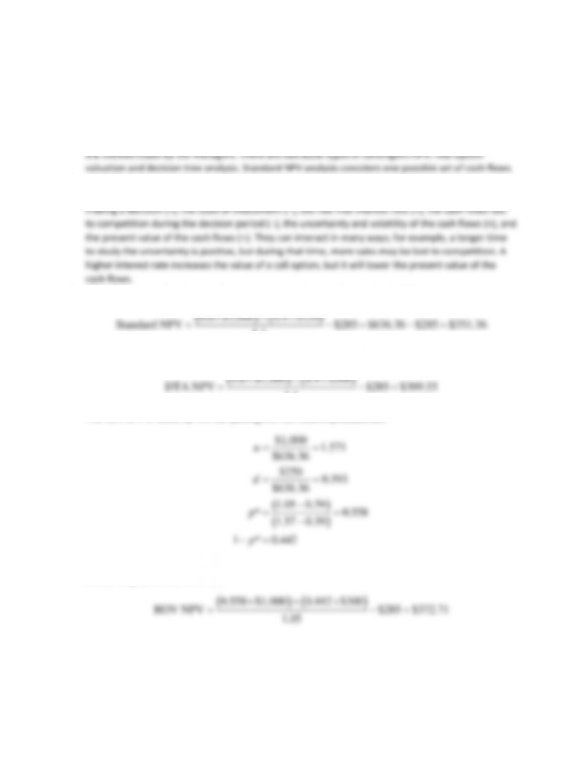
1. Contingent NPV incorporates possible cash flows changing either from exogenous factors or from
2. Flexibility is the main driver of value in the real-option approach, and several inputs determine the
value of the option. Those drivers and their effect on the value of the option are the time until
3. Using the current liquidation value as an opportunity cost, the standard NPV is:
( ) ( )
0.6 $1,000 0.4 $250
+
2
for example, while the DCF value can go up from $636 to $1,000 (+57 percent) or down to $250 (–61
percent).
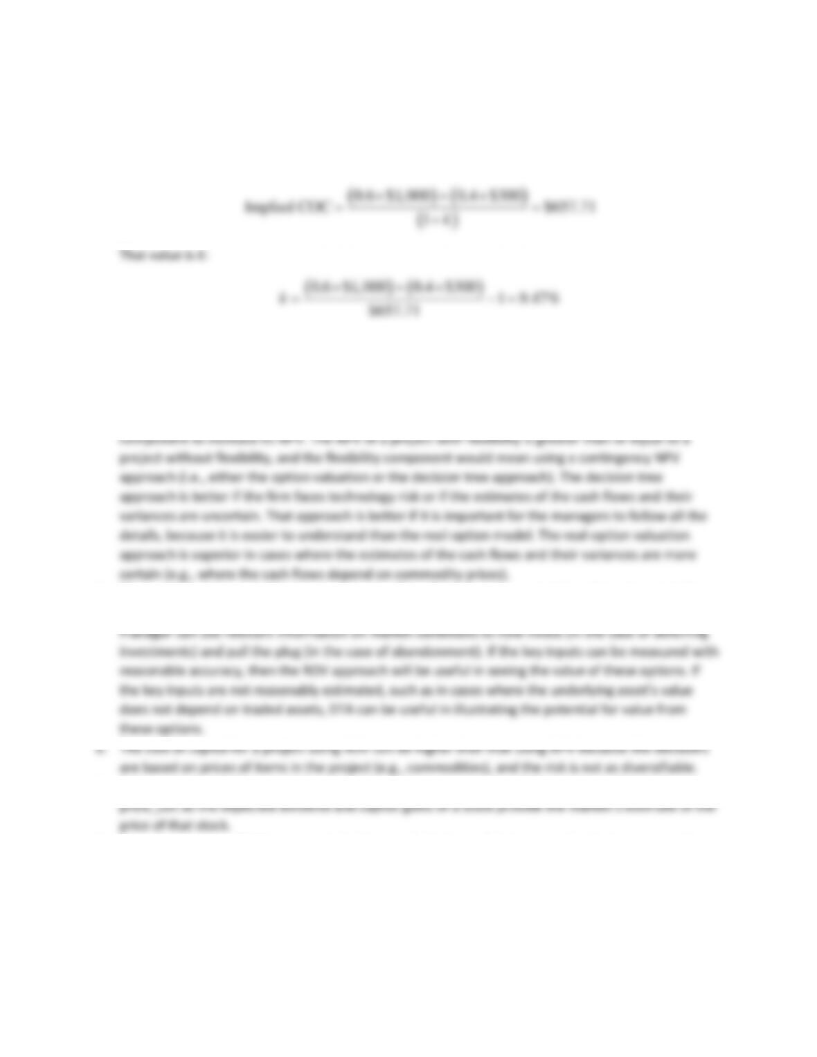
The implied cost of capital when there is flexibility is the value that makes the expected value in the
ROV model equal to the project value, that is, the solution for k in the following expression:
( ) ( )
0.6 $1,000 0.4 $300
+
$657.71
Since this is less than 10 percent, there is an underestimation of project value with flexibility
(although the difference is small).
4. The standard NPV approach applies in a case where there is low uncertainty and/or managers do
not have the ability to make major decisions such as expansions or terminations as information
arrives in the future. If the NPV of a project is close to zero, managers may wish to add a flexibility
5. These two options mean the manager can significantly reduce the probability of negative cash flows
and stop a project where the liquidation value exceeds the discounted estimated cash flows. A
7. The expected cash flows provide an estimate of the present value of the project, which is like a
8. Since the nondiversifiable commercial risk was relatively small in the example, the two approaches
delivered the same estimate of NPV = $120 million. For some sufficiently large level of commercial
risk and assuming the other inputs (e.g., the value of the completed drug) remain constant, ROV
NPV will be higher than ROV DTA, since the lower limit of value will not change, but the increase in
volatility will increase the positive values. How high must the volatility be to make the ROV NPV
higher than the DTA NPV? A trial-and-error search can find the value for volatility where the two

3