Unlock document.
This document is partially blurred.
Unlock all pages and 1 million more documents.
Get Access
points = tfinal/dt + 1;
t = zeros(points,1); r = zeros(points,1);
for i=1:points,
t(i)=(i-1)*dt;
% reference model
% NN inputs
% get weights from state vector
% adaptive controller
else u(i) = u_sl;
end
% reference model modified
rdot = vrm - vh;
% learning law
figure(1)
subplot(2,1,1)
plot(t,[r x(:,1) r(:,1)]);
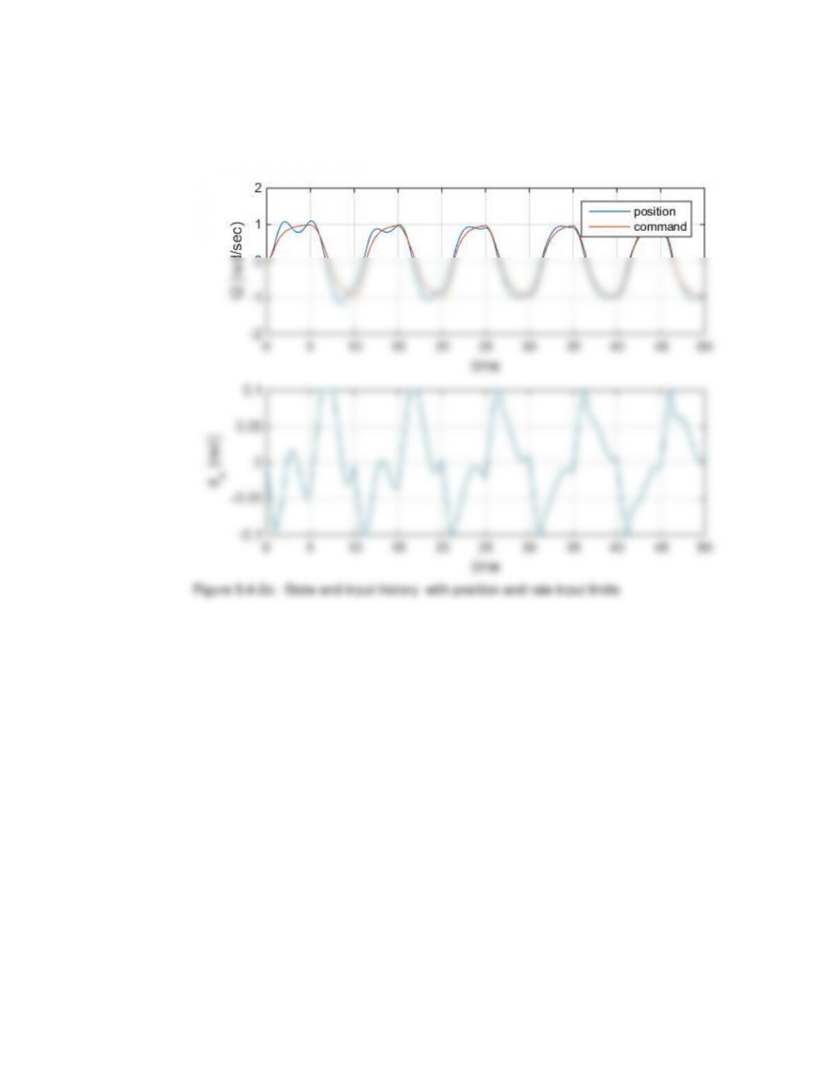
xlabel('time');
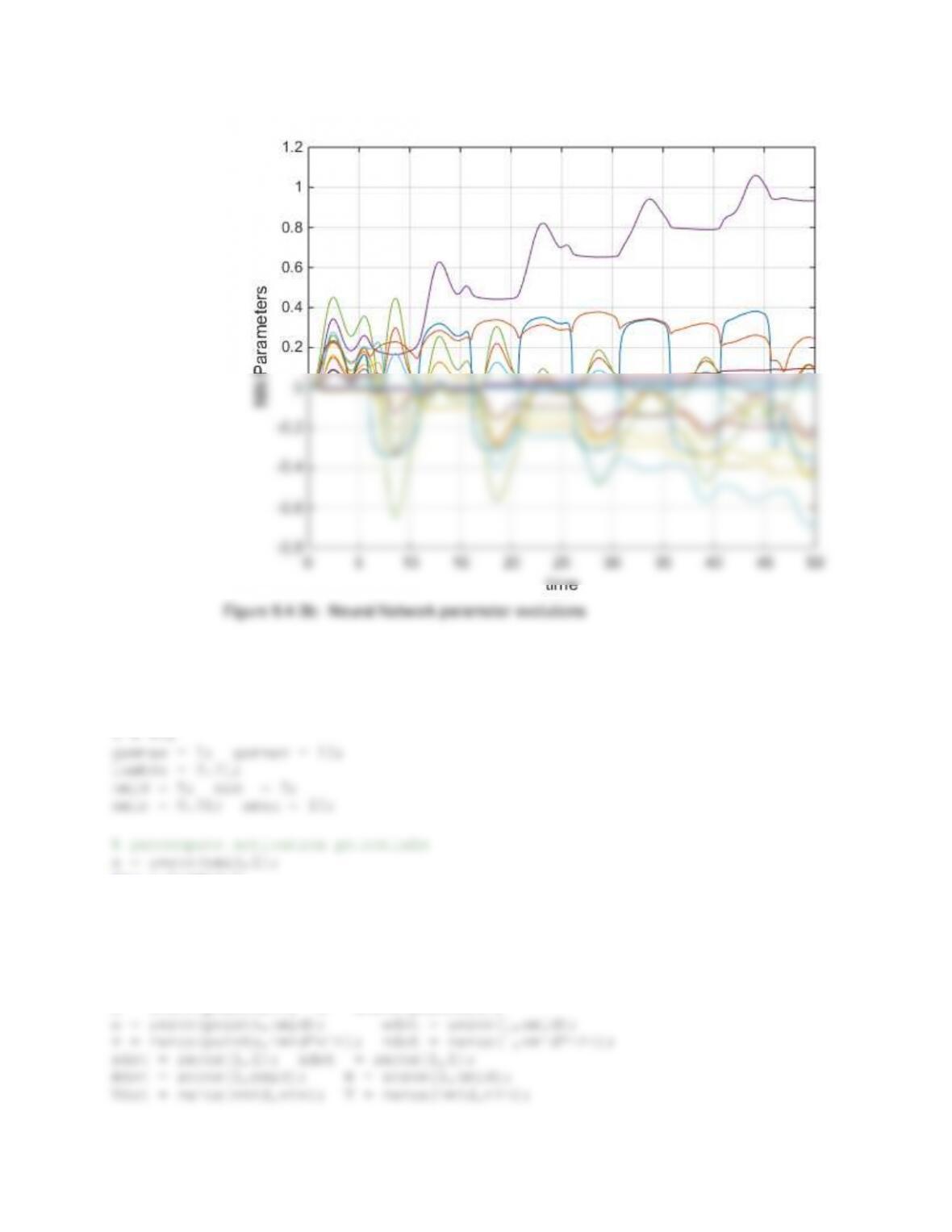
ylabel('NN Parameters');
grid;
Problem 9.4-3: MATLAB script of implementation:
% preallocate arrays
% get weights from state vector
W = w(i,:);
sigp(j,j) = a(j)*ez*sig(j)*sig(j);
end;
sig(nmid) = 1;
vad = W*sig;
vv = vrm - K*e - vad;
ebest = abs(u_allowed(j)-u_cmd);
jbest = j;
end;
end;
u(i) = u_allowed(jbest);
Wdot = -gammaw*( e*( sig' - xbar'*V'*sigp ) + lambda*norm( e )*W );
Vdot = -gammav*( sigp*W'*e*xbar' + lambda*norm( e )*V );
% put NN update in a vector
wdot = Wdot;
% numerically integrate
if i==1,
x(i+1,:) = x(i,:) + xdot*dt;
r(i+1,:) = r(i,:) + rdot*dt;
ylabel('Q (rad/sec)');
legend('position','command');
grid;
subplot(3,1,2)
plot(t, u(:,1) );
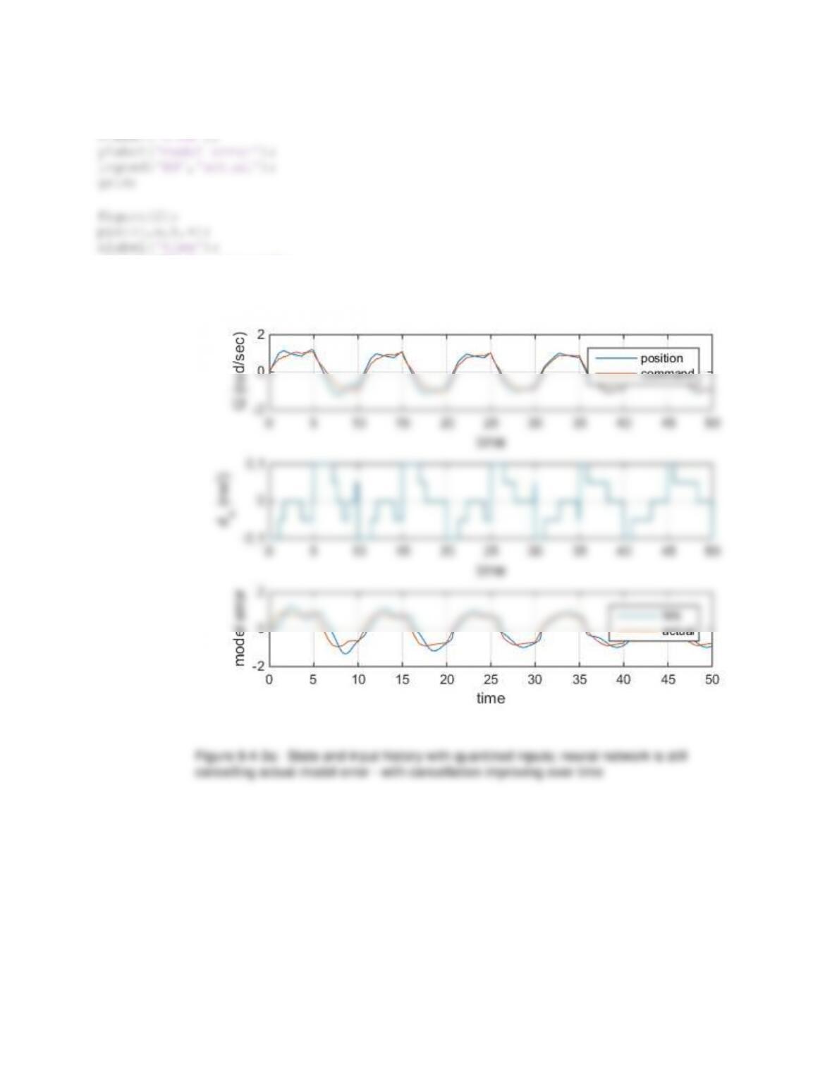
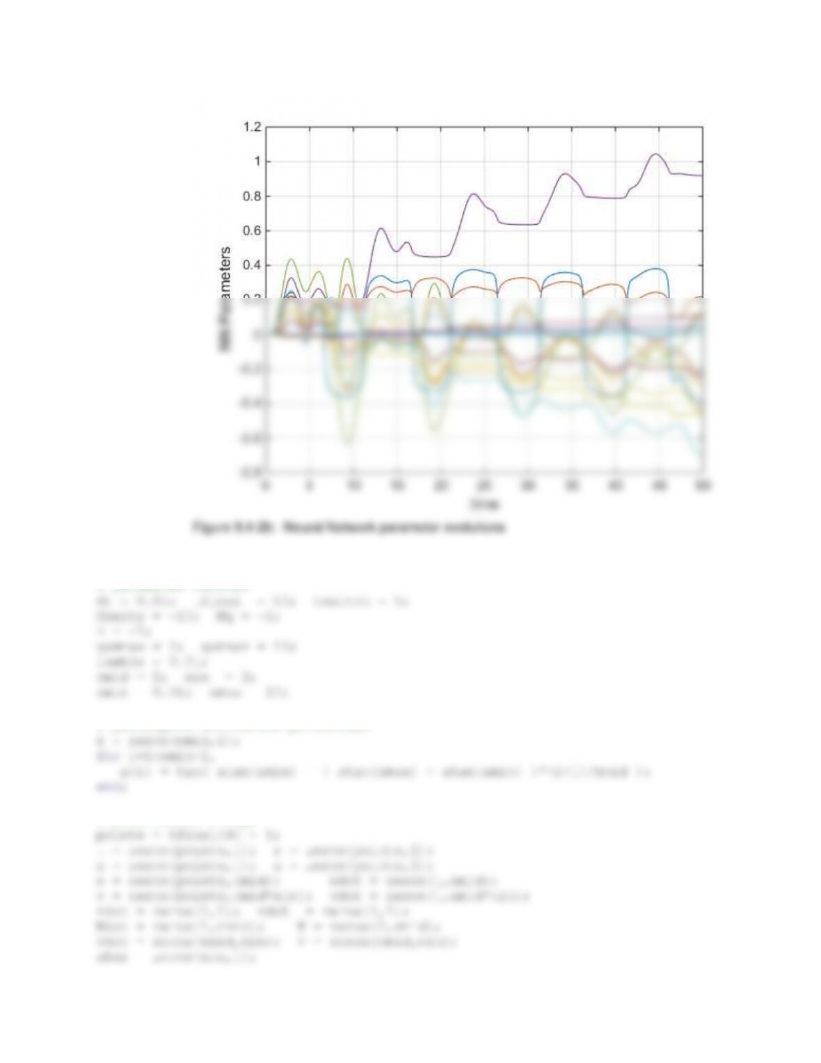
subplot(3,1,3)
plot(t, vad_save, t, Delta_save );
ylabel('NN Parameters');
grid;
Problem 9.4-4: MATLAB script of implementation:
% parameter choices
dt = 0.05; tfinal = 50; tswitch = 5;
Mdelta = -10; Mq = -1;
for i=1:nmid-1,
a(i) = tan( atan(amin) + ( atan(amax) - atan(amin) )*(i+1)/nmid );
end;
% preallocate arrays
points = tfinal/dt + 1;
t = zeros(points,1); r = zeros(points,1);
x = zeros(points,1); u = zeros(points,1);
% external input
if mod(t(i),2*tswitch)<tswitch, externalInput = 1;
else externalInput = -1;
end;
% reference model
vrm = -K*( externalInput - r(i,1) );
V(j,:) = v(i,(j-1)*nin+1:j*nin);
end;
% adaptive controller
vx = V*xbar;
for j=1:nmid-1,
ez = exp( -a(j)*vx(j) );
% plant model
xdot = sin( x(i,1) ) + Mdelta*u(i) + Mq*x(i,1);
% hedge signal
fhat = Mdelta*uhat + Mq*x(i,1)
vh = vv - fhat;
vdot((j-1)*nin+1:j*nin) = Vdot(j,:);
end;
% save for plotting purposes
vad_save(i) = vad;
Delta_save(i) = xdot - fhat;
% numerically integrate
if i==1,
x(i+1,:) = x(i,:) + xdot*dt;
end;
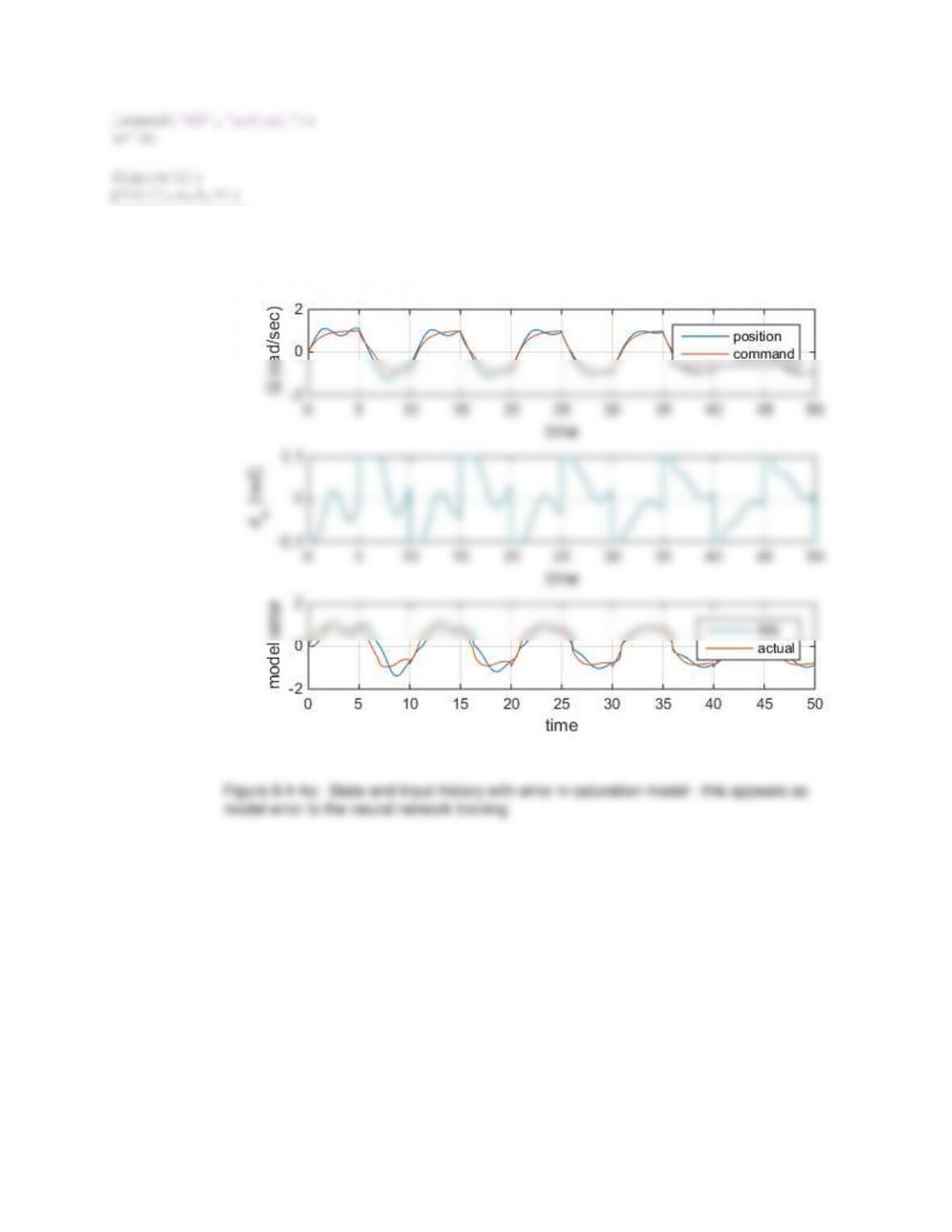
figure(1)
subplot(3,1,1)
plot(t,[x(:,1) r(:,1)]);
xlabel('time');
ylabel('d_e (rad)');
grid;
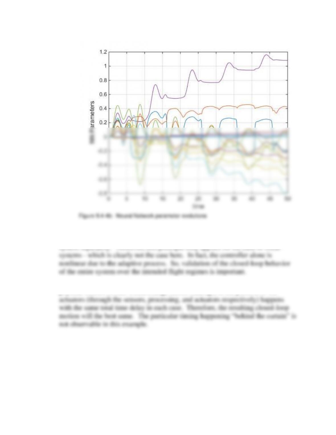
subplot(3,1,3)
xlabel('time');
ylabel('NN Parameters');
grid;
Problem 9.5-1: (quoting Section 9.5) From Section 6.4 we find that the separation
principle justifies designing the guidance/control system and the state estimation
system separately. However, this principle only applies for the case of linear
Problem 9.5-2: From the perspective of the aircraft itself, the communication of aircraft
physical motion (which would change sensor readings) to the position of the
Problem 9.5-3: To the extent that the adaptive controller is intended to correct for model
error in flight, any training occurring while on the ground could potentially reduce
performance after leaving the ground. Worst case, adaptation could “wind up”
Problem 9.5-4: This is a case where adaptation likely has enough performance to
address changes with flight condition. This is partially enabled by the fact that


