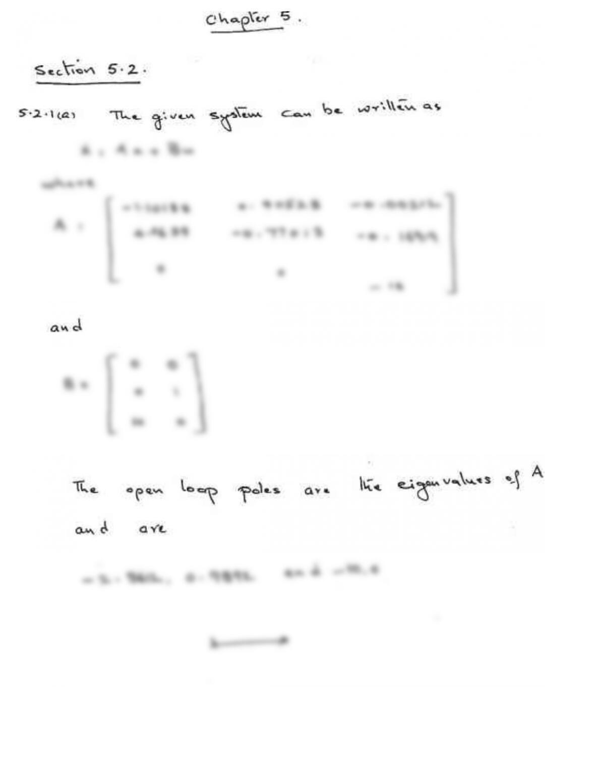
0.0021499,0,0,0,0,0,-0.00025384,-1.0189,0,0.90506,0,0,0,0;
0,0,0,0,0,0,0,0,0,1,0,0,0,0;
0.17555,0,0,0,0,0,2.9465e-012,0.82225,0,-1.0774,0,0,0,0;
command
if i==0
Cp= [zeros(1,12),57.29578,0]; % roll-rate
Cq= [zeros(1,9),57.29578,0,0,0,0]; % pitch-rate
Cy= [zeros(1,12),0,57.29578]; % yaw-rate
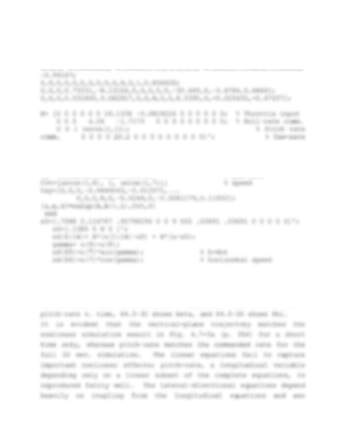
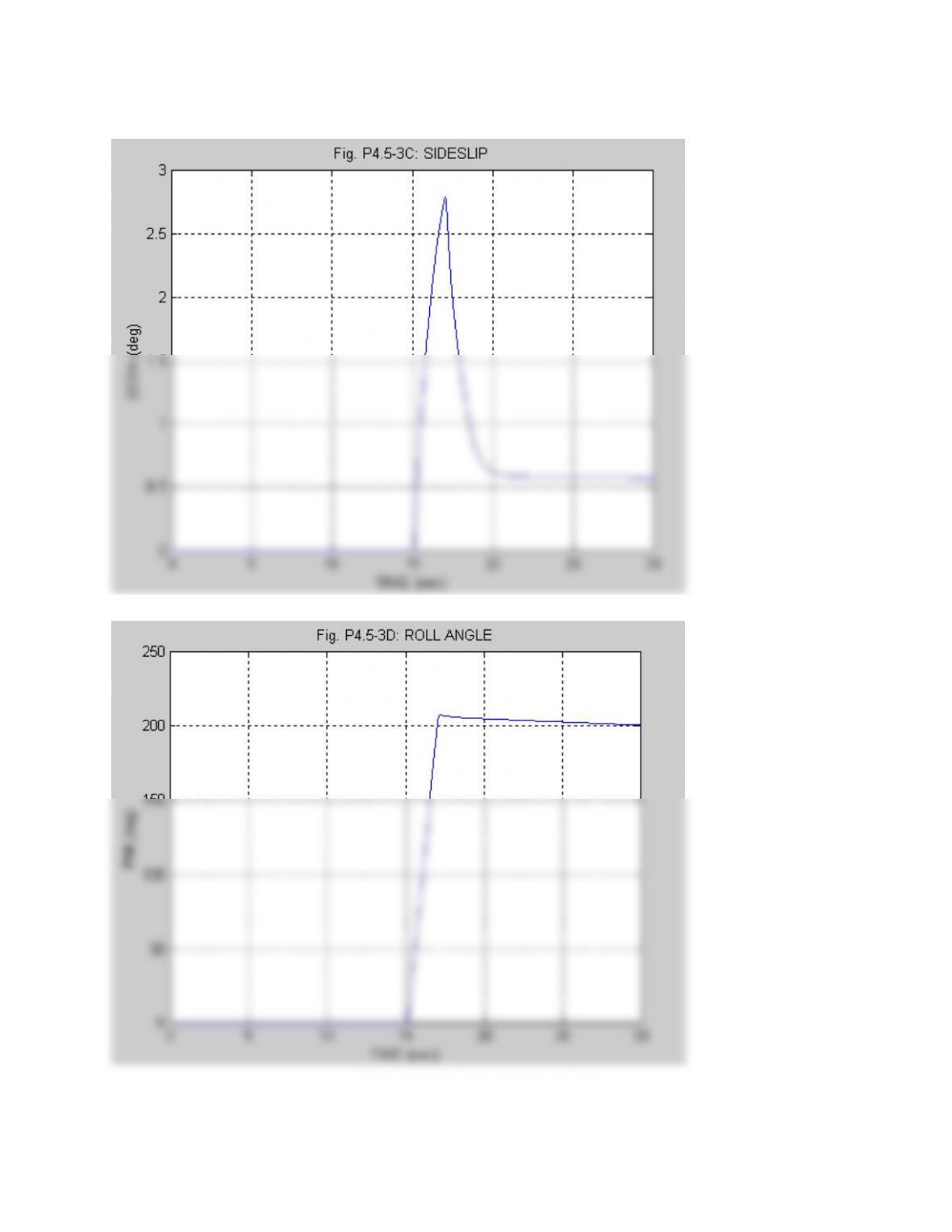
(b) Maneuvers can conveniently be simulated by programming into
NLSIM the same commands that were used in Ex. 4.7-2. Figure
P4.5-3A shows the vertical-plane trajectory, Fig. P4.5-3B shows
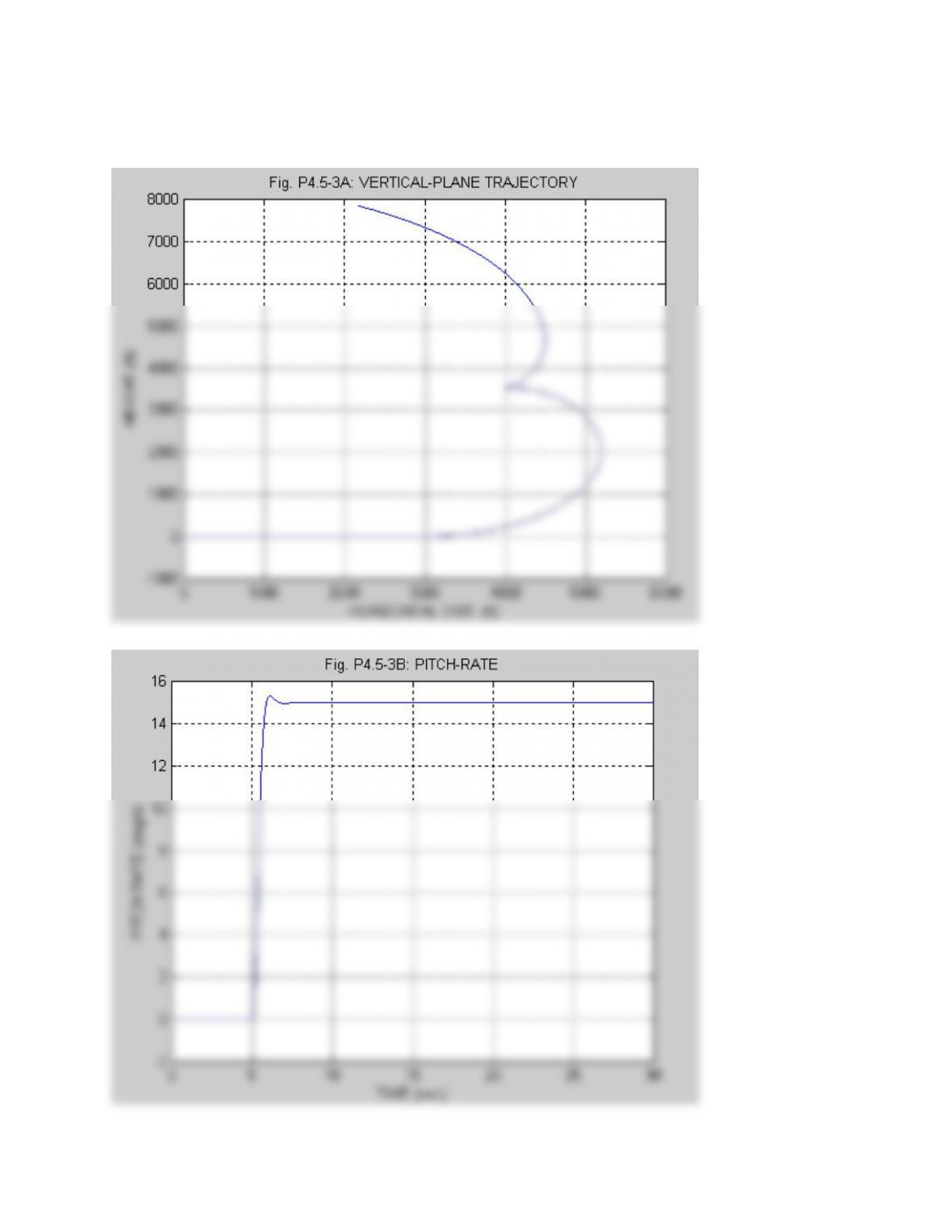
unlikely to work well.
————————
Problem 4.6-1: Transport aircraft pitch-attitude-hold re-design.
For the short period approximation, take only the alpha and
pitch-rate states from the coefficient matrices in Ex. 4.6-1 and
add an integrator. The code is shown below:
% PROBLEM 4.6-1 (EXAMPLE 4.6-1 PITCH-ATTITUDE HOLD)
clear all
asp=[-.56761 1.0; -1.4847 -.47599];
The closed-loop pitch-attitude transfer function obtained
from this code is:
which closely matches transfer function (3) in Ex. 4.6-1 when the
phugoid poles and nearby zeros are removed from that transfer
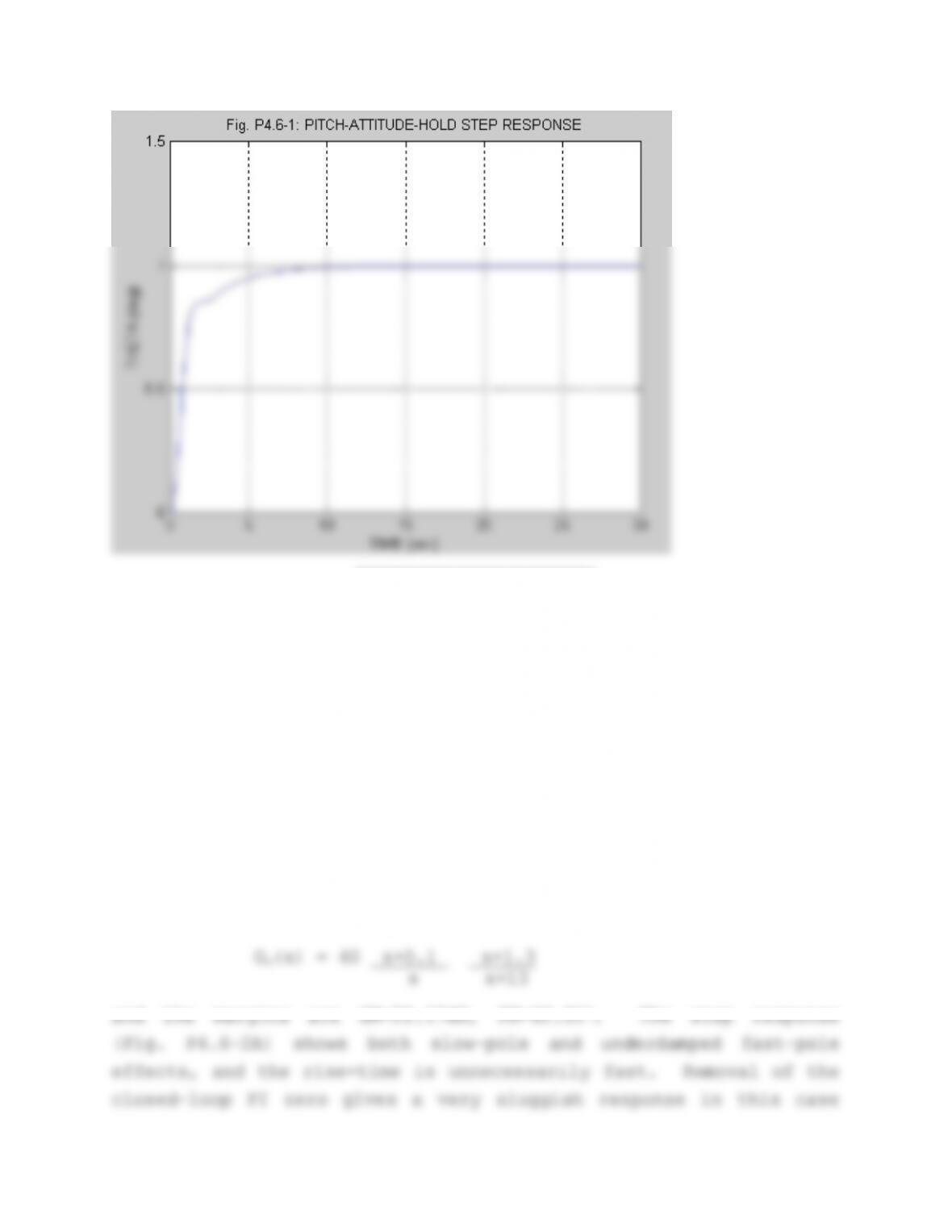
———————-
Problem 4.6-2: Pitch-attitude hold with dynamic compensation.
Follow the same procedure as in Ex. 4.6-2, using the 4-state
longitudinal dynamics equations (altitude state omitted), with the
PI zero at s=-0.1. Fix the compensator gain at a convenient value
(e.g. k=40), the lead compensator pole-zero ratio at p/z =10, and
adjust the compensator pole position to obtain the maximum phase
margin.
Increasing the pitch-rate feedback, kq, tends to increase the
gain and phase margins, and a value kq=0.6 provides adequate
margins. The phase margin is then maximized, with an adequate
gain margin, by the compensator:
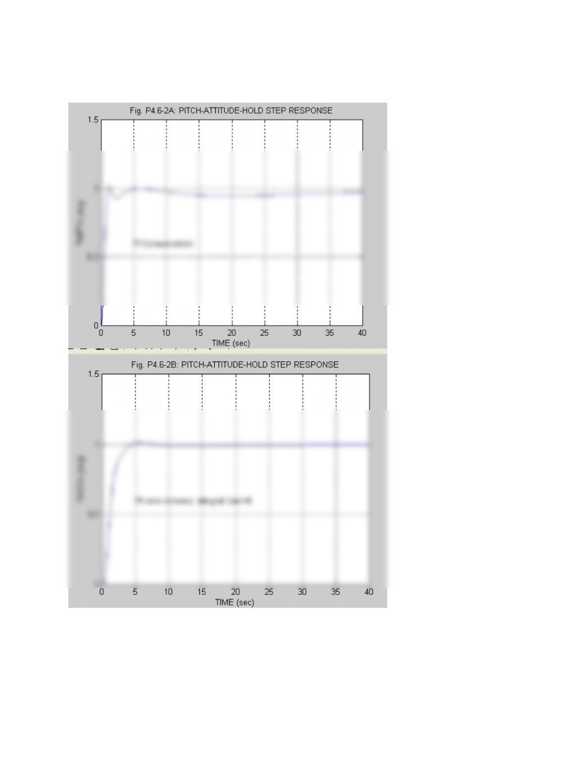
but, if the integral gain is then increased (to about 8), a very
good step response is obtained
. Figure P4.6-2B shows this response, with the system arranged
for unity feedback of theta.
————————
Problem 4.6-3: Mach-hold for the transport aircraft model.
To get an output matrix for Mach, it is convenient to create
a fake state-derivative in the transport aircraft model (e.g.
xd(7)=M, since “d” is not in use), use the linearization program,
and take the corresponding row of the A-matrix as “CM.” The C-
matrix row and B-matrix column (for δt input) are:
The transfer function from throttle to Mach is found to be:
The short-period poles can be cancelled out of this transfer
4.6-1. With kp=4 and kq=2.5 the throttle to Mach transfer
function becomes:
note that the pole at s=-0.2 is the throttle actuator pole. A
zero and a pole can be cancelled, and a root-locus sketch of the
The step response is rather lightly damped, but the system would
not normally be subjected to step command inputs. Of more
importance might be the steady-state error of this type-0 system.
———-———-
Problem 4.6-4: Redesign of the glide-slope controller, Ex. 4.6-4
Use the code given with Ex. 4.6-4, and change the PI compen-
sator ( x(14) ) to (s+0.1)/s. To make the elevator less active
try reducing the phase-lead pole-to-zero ratio to 5.0. The gain
and phase margins are then rather low unless the PI compensator
proportional gain is reduced from 1.0 to 0.8. The gain and phase
margins versus pole position are as follows:
If p=3 is chosen (by giving more weight to phase margin than gain
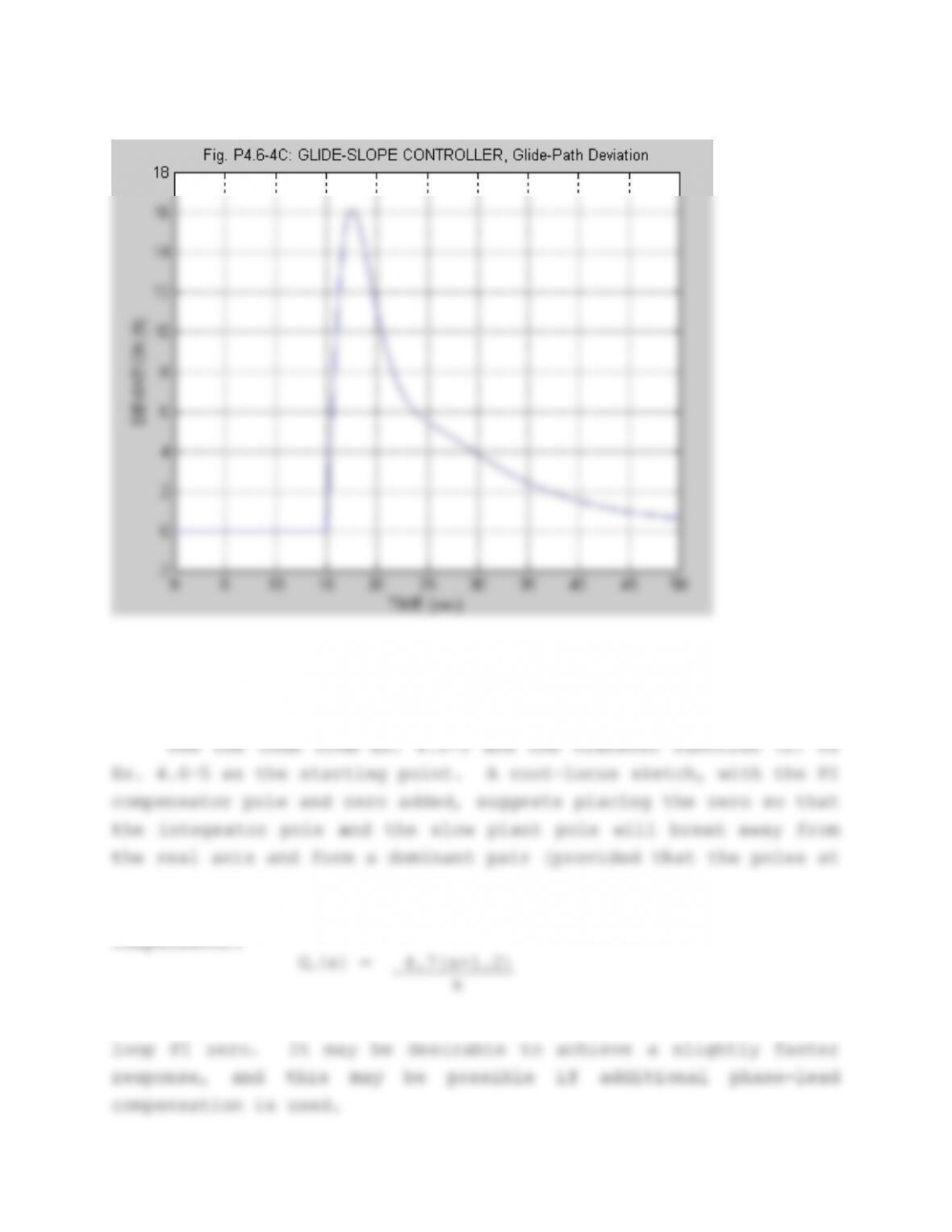
———-———–
Problem 4.6-5: Type-1 control of roll angle, Ex. 4.6-5 modified.
s= -11.8±j11.0 do not move very much to the right).
Root-locus plots and step-response simulation led to the
Figure P4.6-5 shows the step response with and without the closed-
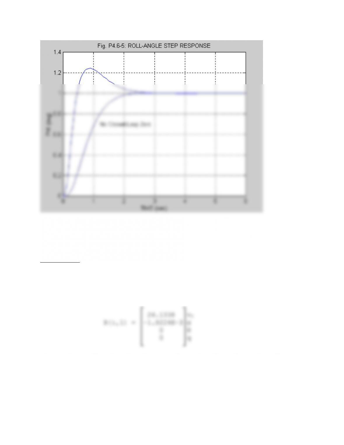
———————–
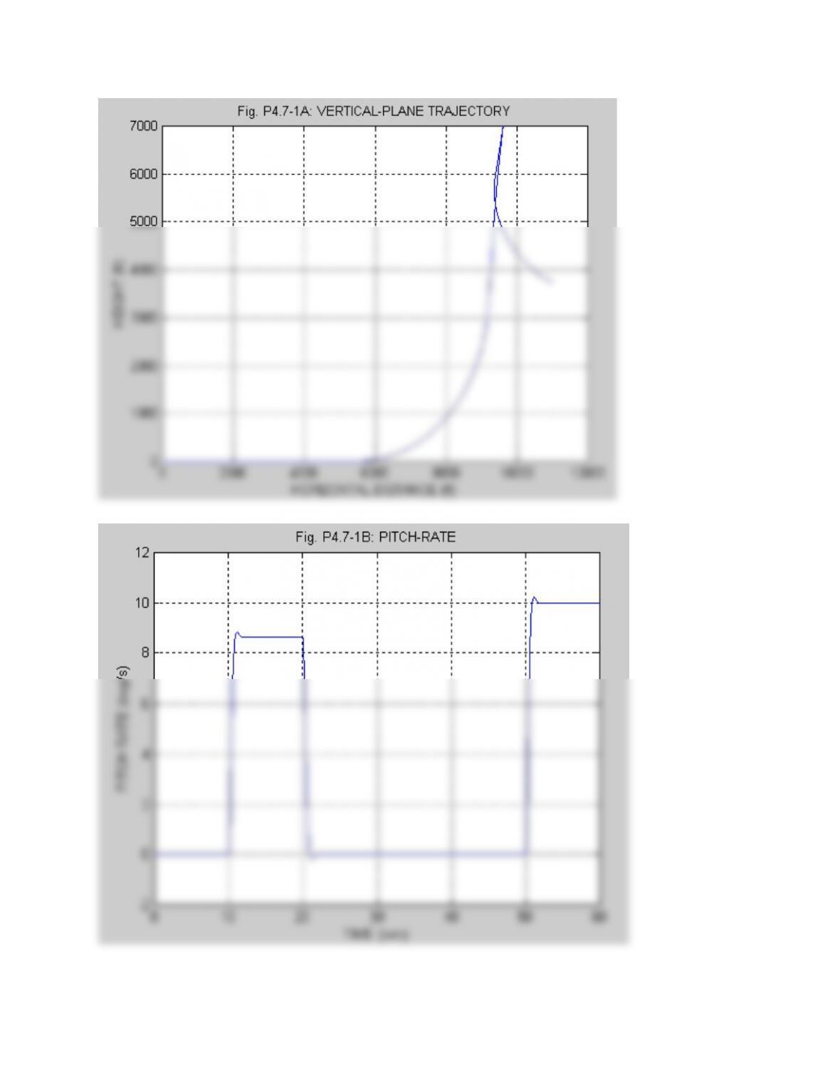
**Problem 4.7-1: Repeat Ex. 4.7-1 with a linear F-16 model.
Correction: The B-matrix for throttle inputs should be provided
(see below).
Using the linear 4-state dynamics (Exs. 4.1-1, 4.4-2, and
4.5-1), add a throttle-input column to the B-matrix:
where the engine lag has been neglected. Now close the elevator
feedback loops as in Ex. 4.5-1, with the closed-loop PI zero
removed. The closed-loop coefficient matrices have been pasted
into the function P471.m shown below.
The linear small-perturbation equations are:
x
. = A(x-Xe) + B(u-Ue)
where the equilibrium state and control vectors can be found from
Table 3.6-3 (p. 197). The equilibrium state of the PI integrator
can be found from,
where q=0 in equilibrium, and 2.1148 is the angle of attack in
degrees. This yields
Thus, the initial state vector is:
In order to plot a trajectory, two more (nonlinear) state
equations will be needed:
.(8) = x(2)sin(x(4)-x(3)) (vertical speed)
x
All of the state equations and initial conditions have been
incorporated in the function P471 given below. This function can
now be numerically integrated with NLSIM.
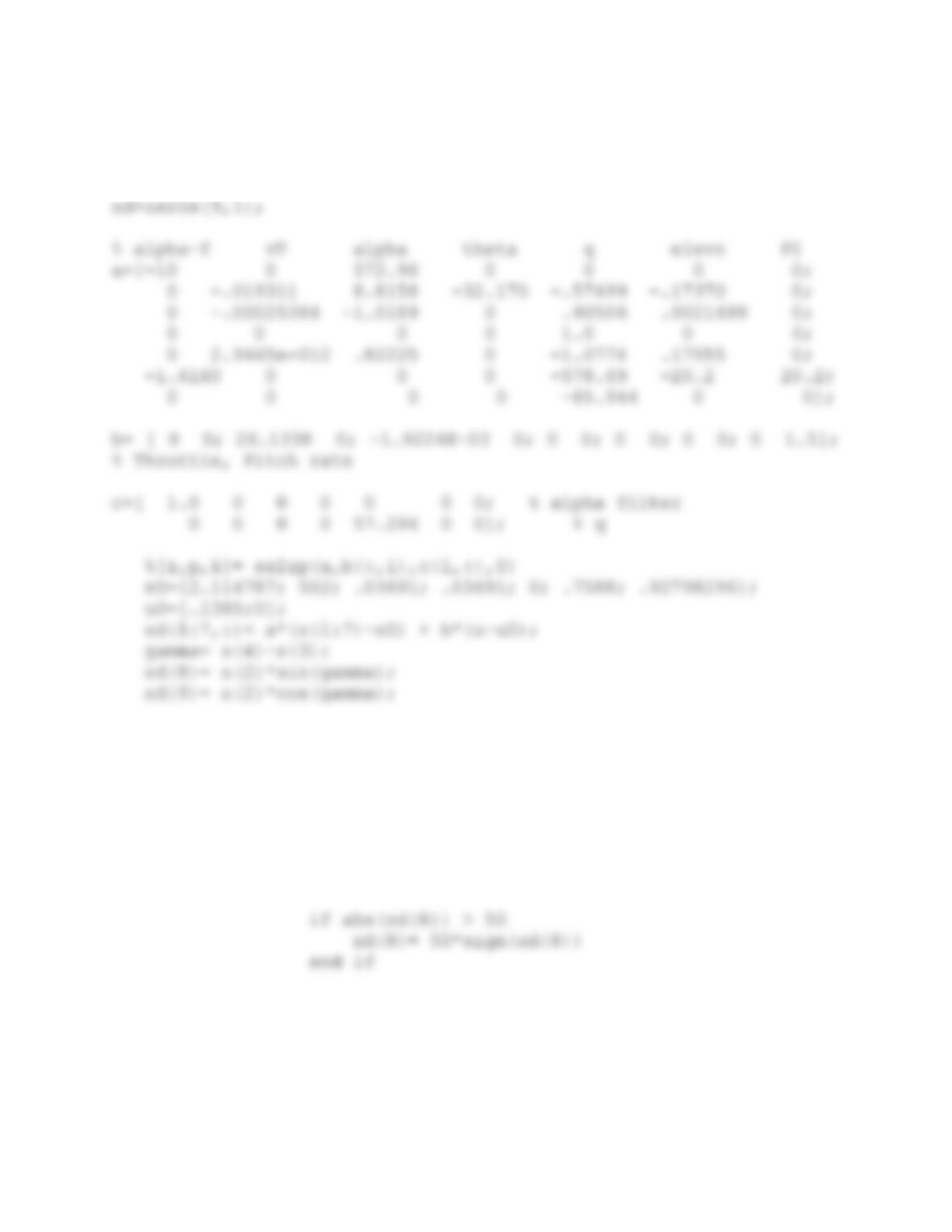
function [xd]= P471(time,x,u)
% PROBLEM 4.7-1 Use Coefficient Matrices from QCAS to get linear
%state eqns.
%clear all
————————
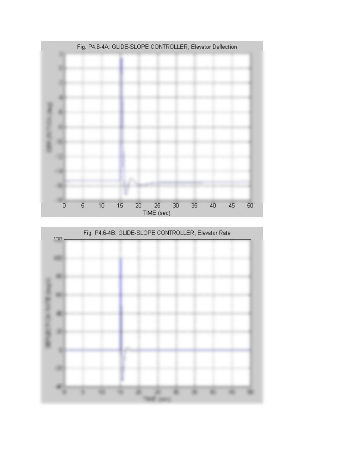
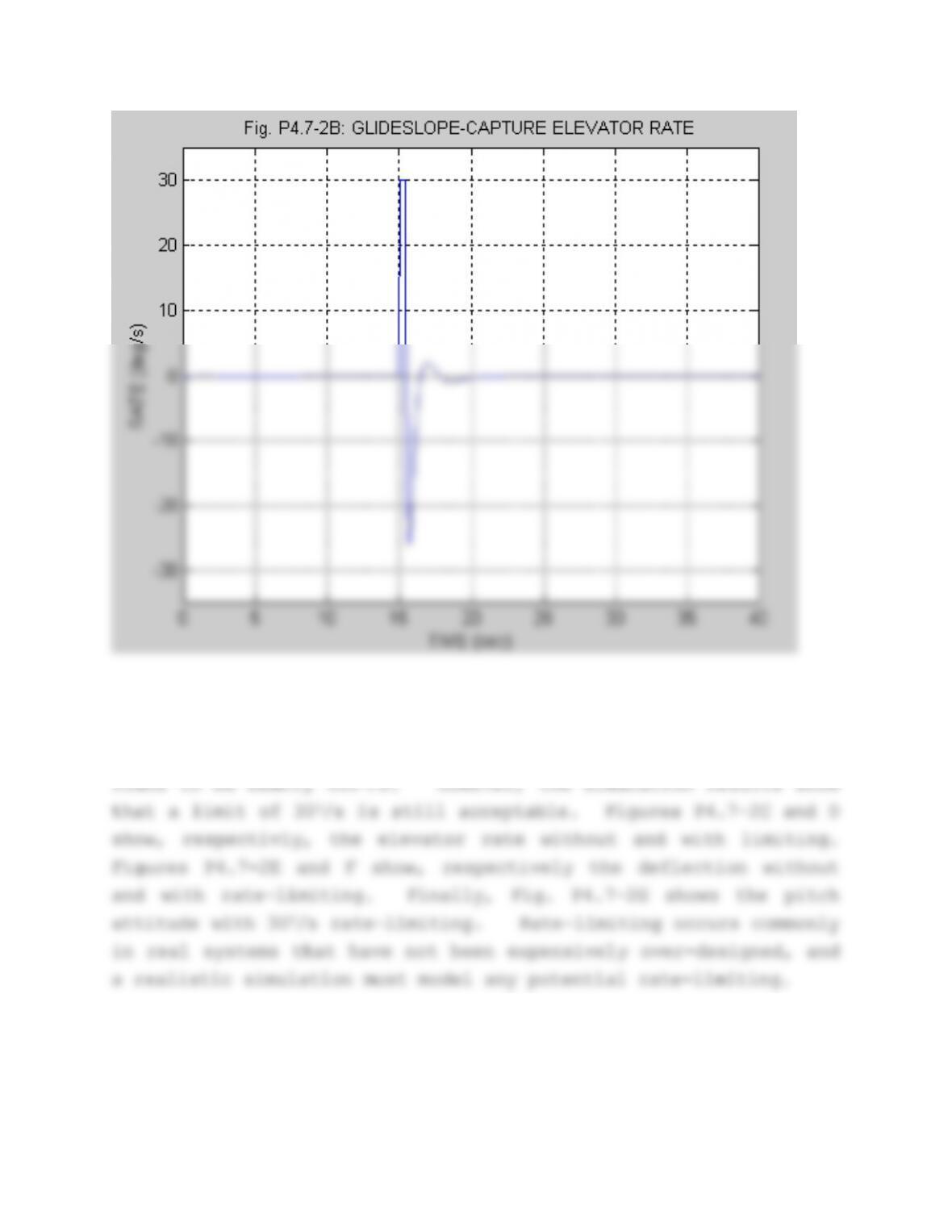
Prob. 4.7-2: Auto. landing simulation with elevator rate-limiting.
To simulate elevator rate-limiting edit the GLIDE and FLARE
functions; after the calculation of the state-derivative xd(8)
insert, for example:
which limits the deflection rate to 50 deg./s. The simulation
time-step should be small enough to accurately reproduce the hard
limit effects. Trial and error can be used to see if the time
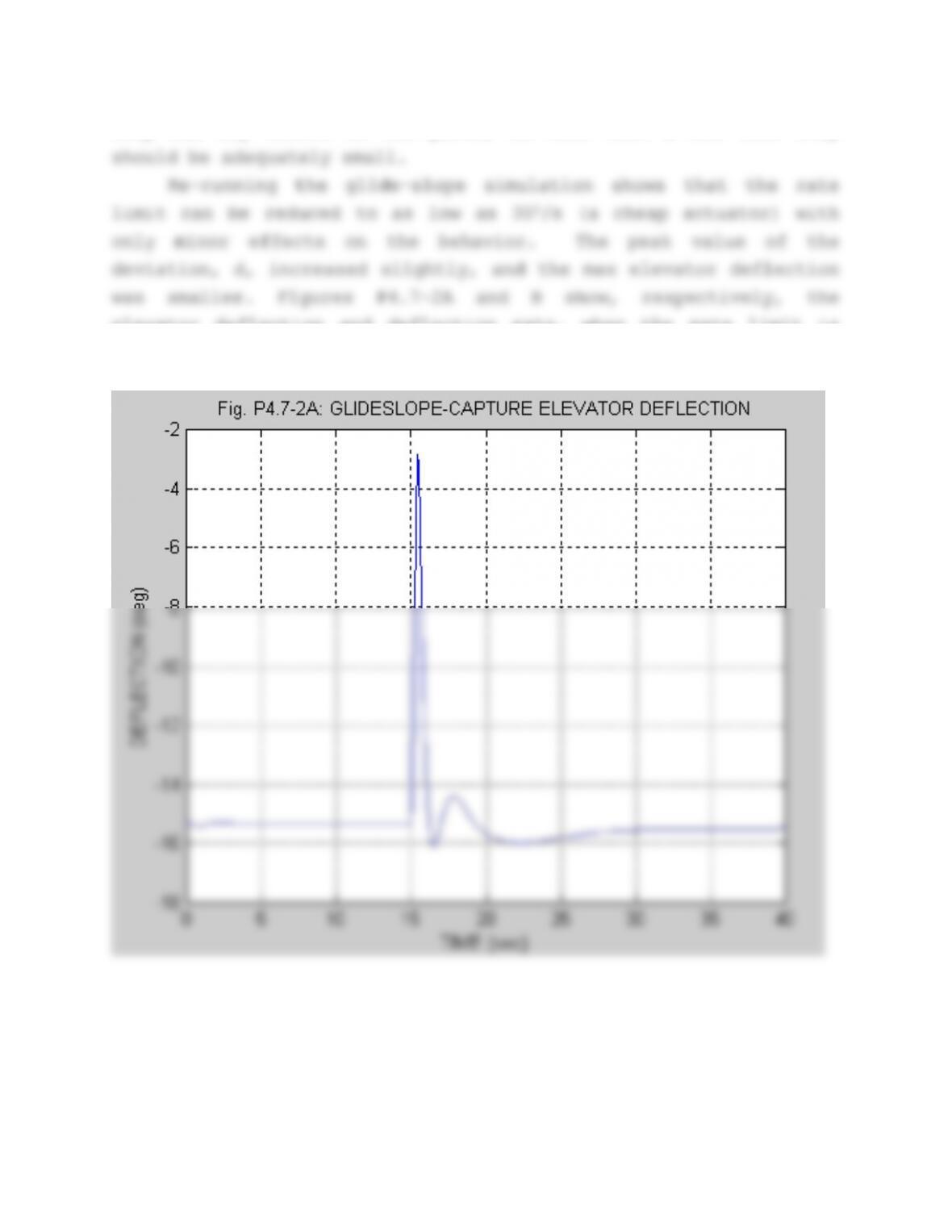
step has any effect on the plots; in this case a 5ms time step
elevator deflection and deflection rate, when the rate limit is
set to 300/s.
The flare simulation may be expected to be more susceptable
to rate limiting since it involves tighter control (i.e. wider
bandwidth and/or higher gains), and the unlimited elevator rate is
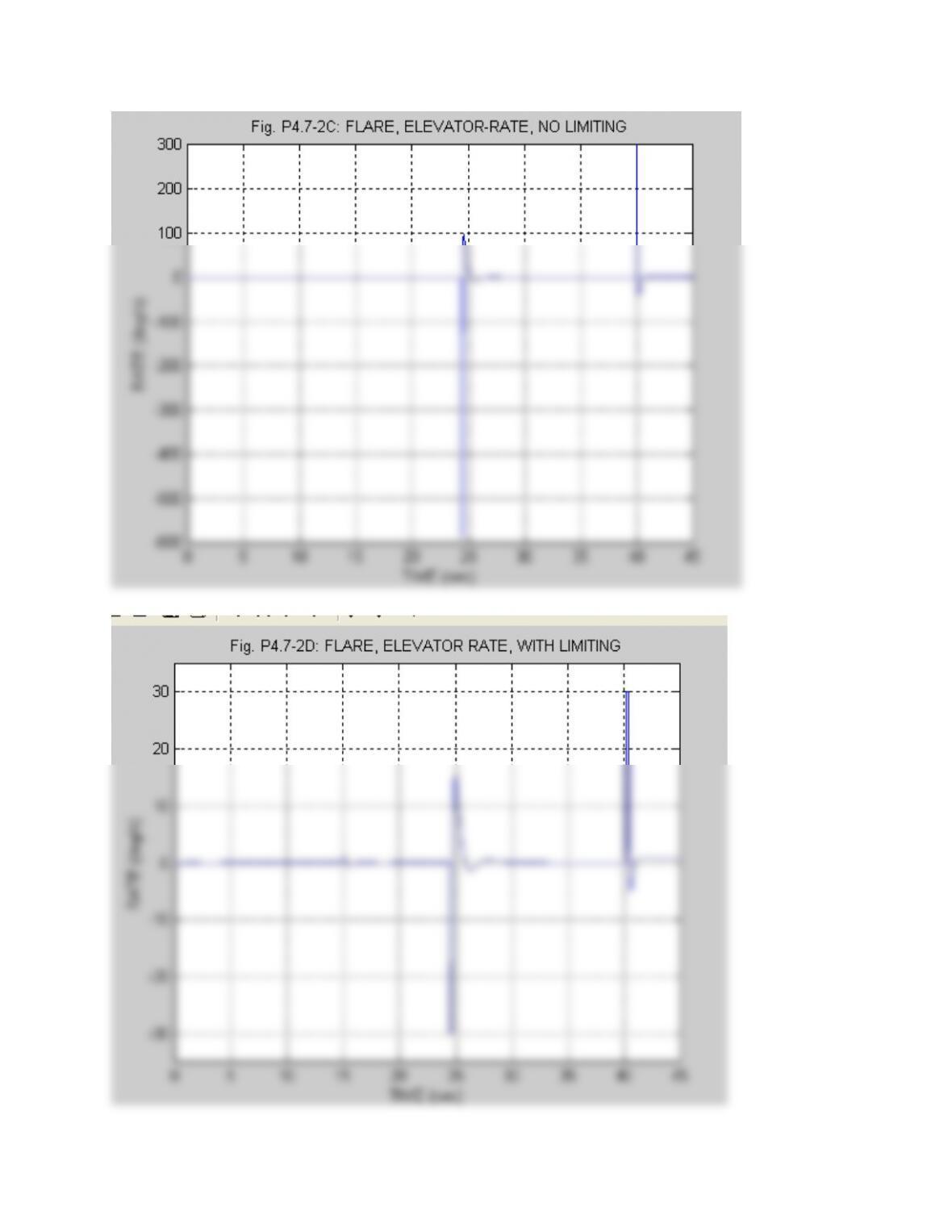
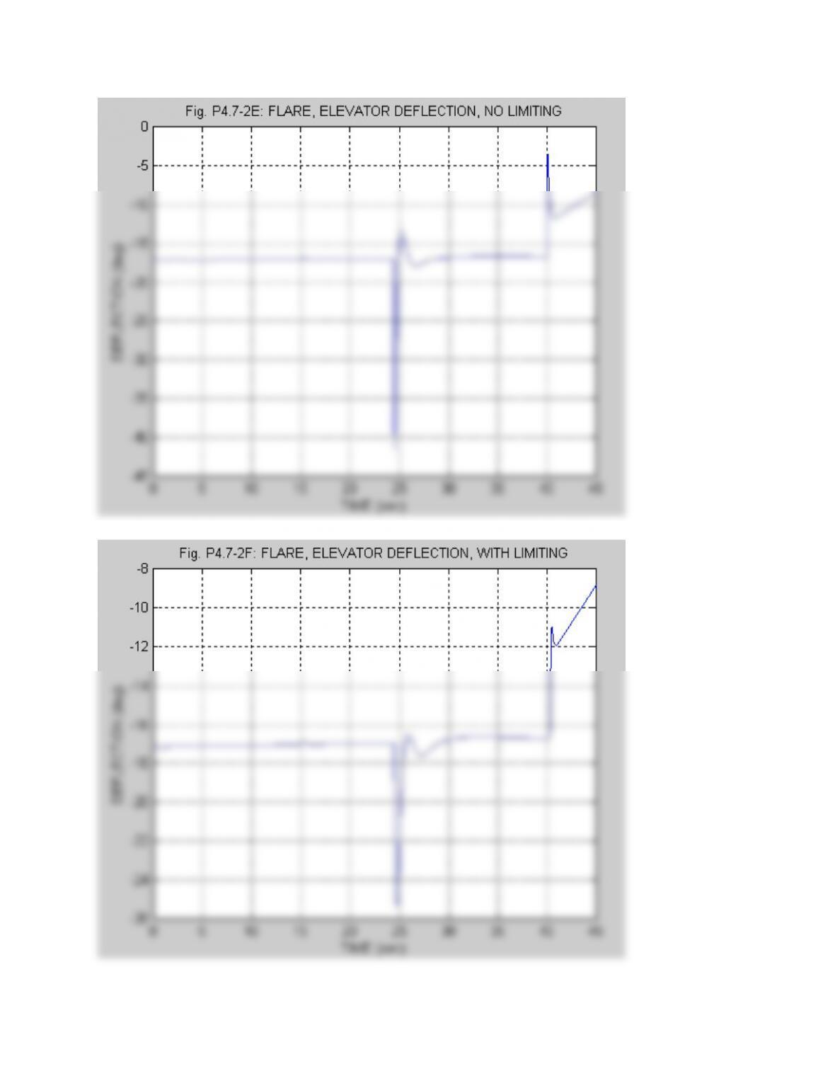
———————-