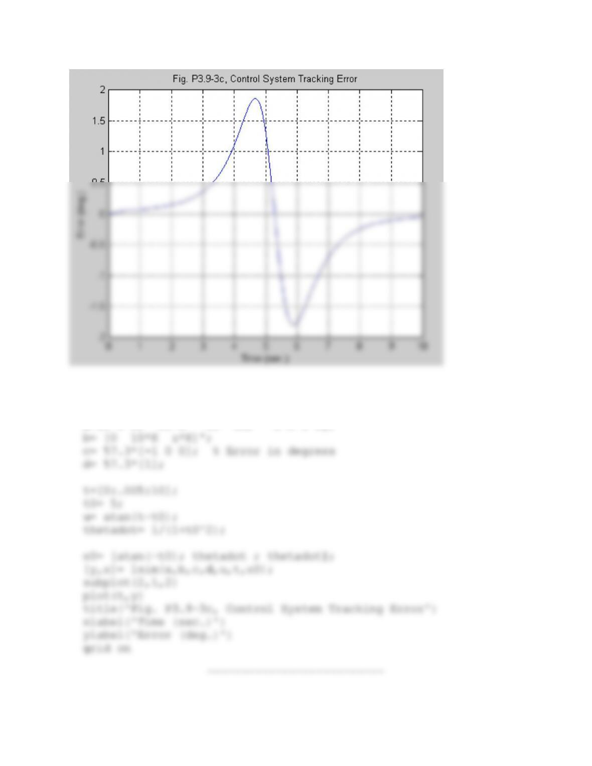
%PROBLEM 3.9-3. Antenna azimuth control for tracking
clear all
z= 2.5; K= 7.6;
a=[0 1 0; -10*K -10 10; -z*K 0 0];
Problem 3.9-4: Stability condition for Ex. 3.9-1
As noted in the example, we must solve for ω1, the higher of the
two frequencies at which Im{G(jω)H(jω)}=0, and then find the value
of K for which Re{G(jω1)H(jω1)}= -1.
Putting s=jω, we obtain,
Now rationalize this and equate the imaginary part to zero:
Solve the quadratic equation in ω2 and take the higher value of ω:
Equating this to -1 gives,
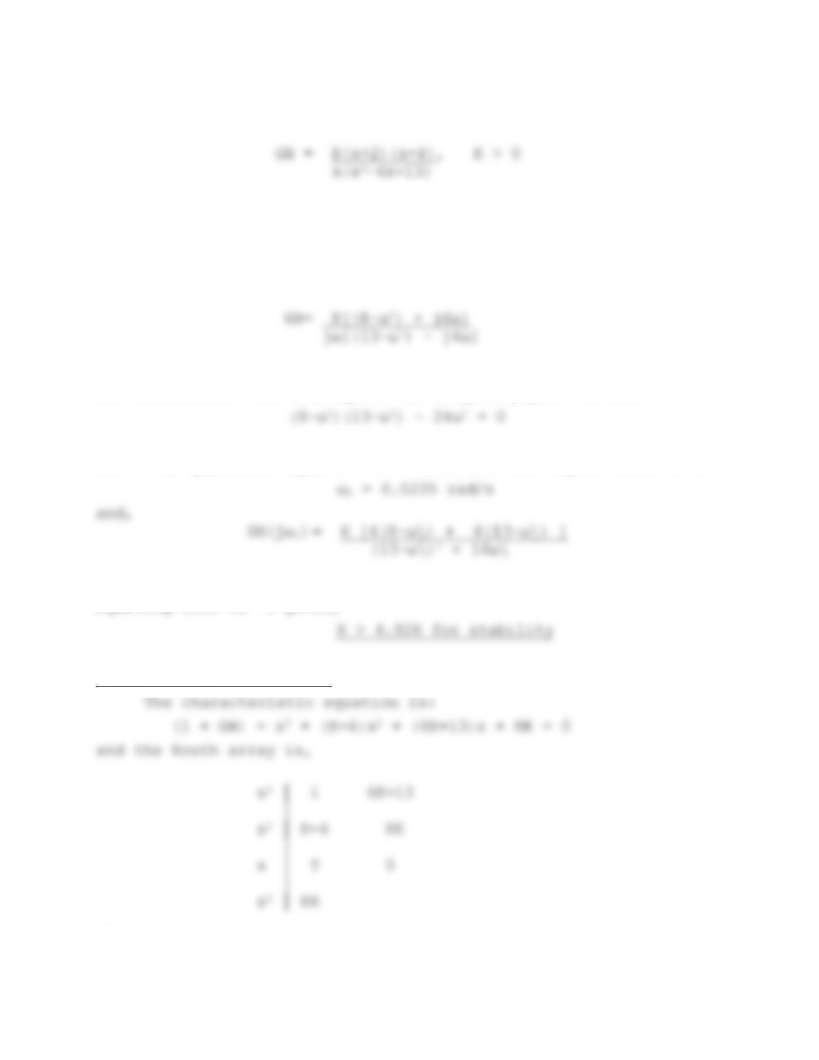
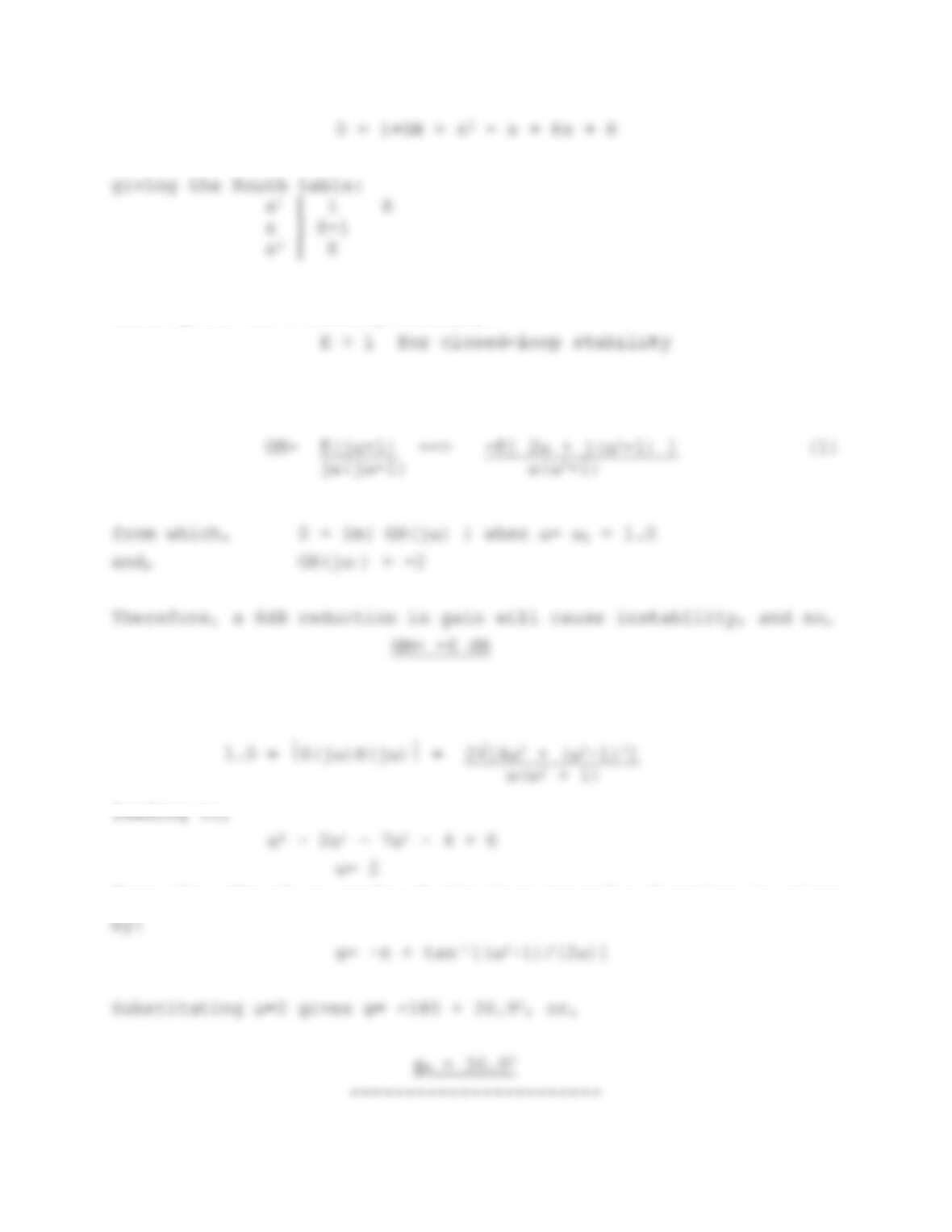
Stability by Routh’s test
where,
The conditions for no sign changes in the first column are:
and so the condition for stability is,
————–————
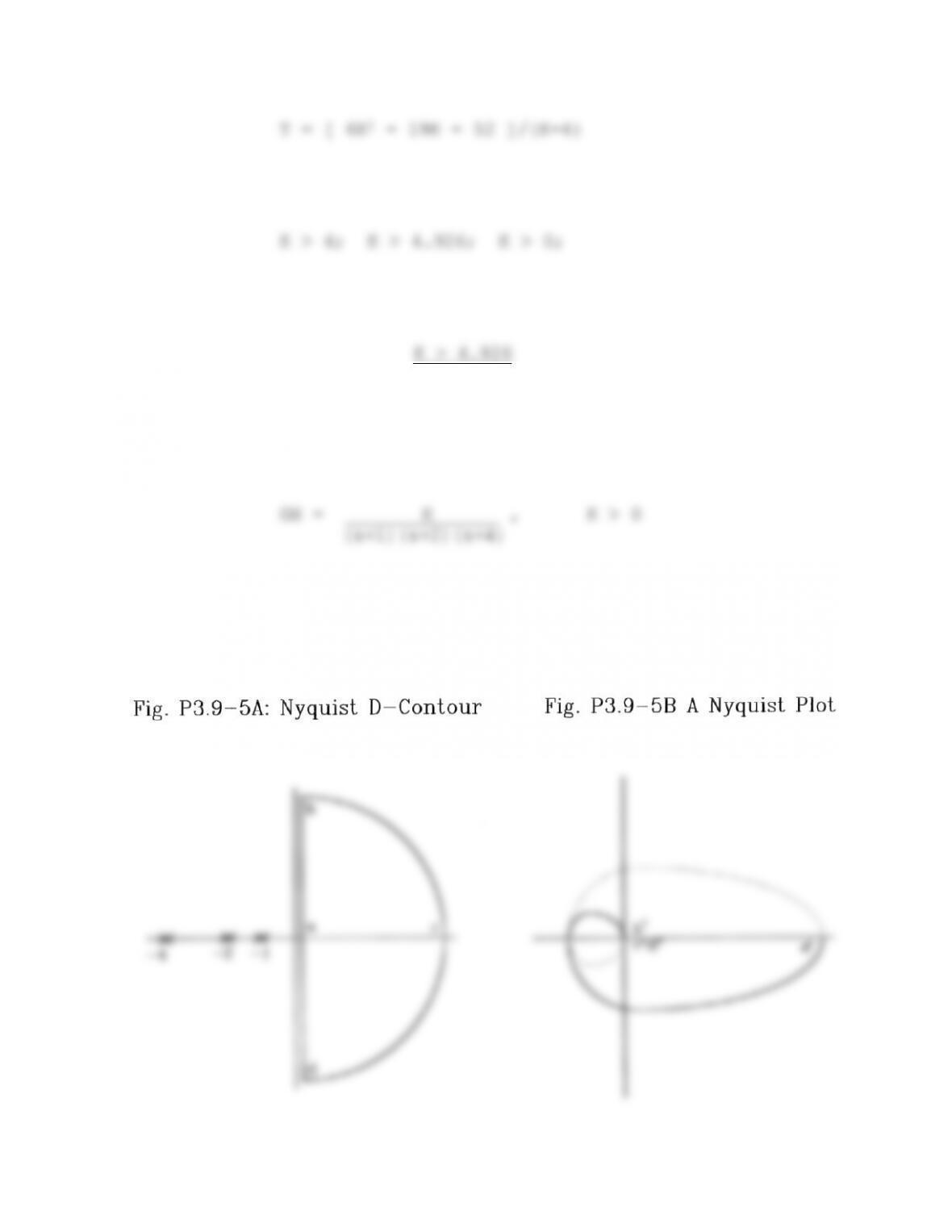
Problem 3.9-5:
(a)Perform the Nyquist test for:
The D-contour and Nyquist plot are shown in Fig. P3.9-5. They show
that there are two unstable closed-loop poles for K greater than
some positive value K1 (Z=P-N = 0-(-2)= 2 )
(b) Find the stability boundary.
Substitute s=jω in G(s)H(s),
———————–
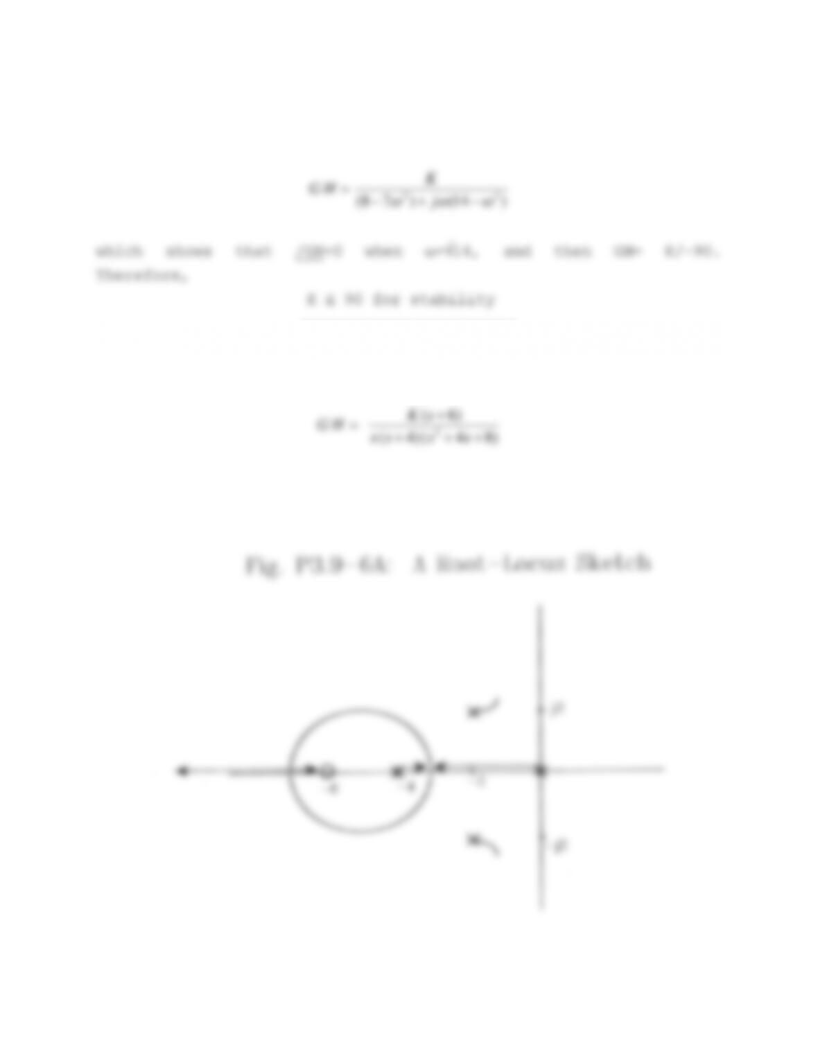
Problem 3.9-6: Root-locus example.
)6(
2
sK
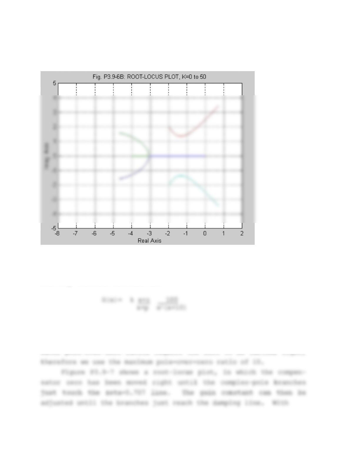
Rules 1 through 4, 6, 7, and 10 allow us to draw the sketch shown
in Fig. P3.9-6A.
In this sketch, we can not be certain which way the complex poles
move (from -2±j2). They are unlikely to move left, while the
other closed-loop pair move right, because the zero at s=-6 is
relatively far away. More information can be obtained by
calculating by calculating their angle of departure, and the root-
locus asymptotes (see below).
(b) Break points and asymptotes:
The characteristic equation gives,
and the real-axis break points satisfy 0= K/s, or,
φ = -63.430
Note that angles can be measured from the computer VDU, or printer
output, if the graph scales are chosen to cancel the usual 4:3
pair from (-2±j2) move into the right-half plane well before the
other complex pair again become real.
———-———-
Problem 3.9-7: Re-design of Ex. 3.9-2.
The loop transfer function is:
By placing a constant-damping line on the root-locus plot we
find that greater damping of the complex pole-pair requires that
the compensator zero be moved to the right. Also, lower compen-
sator pole-over-zero ratios require the zero to be farther right,
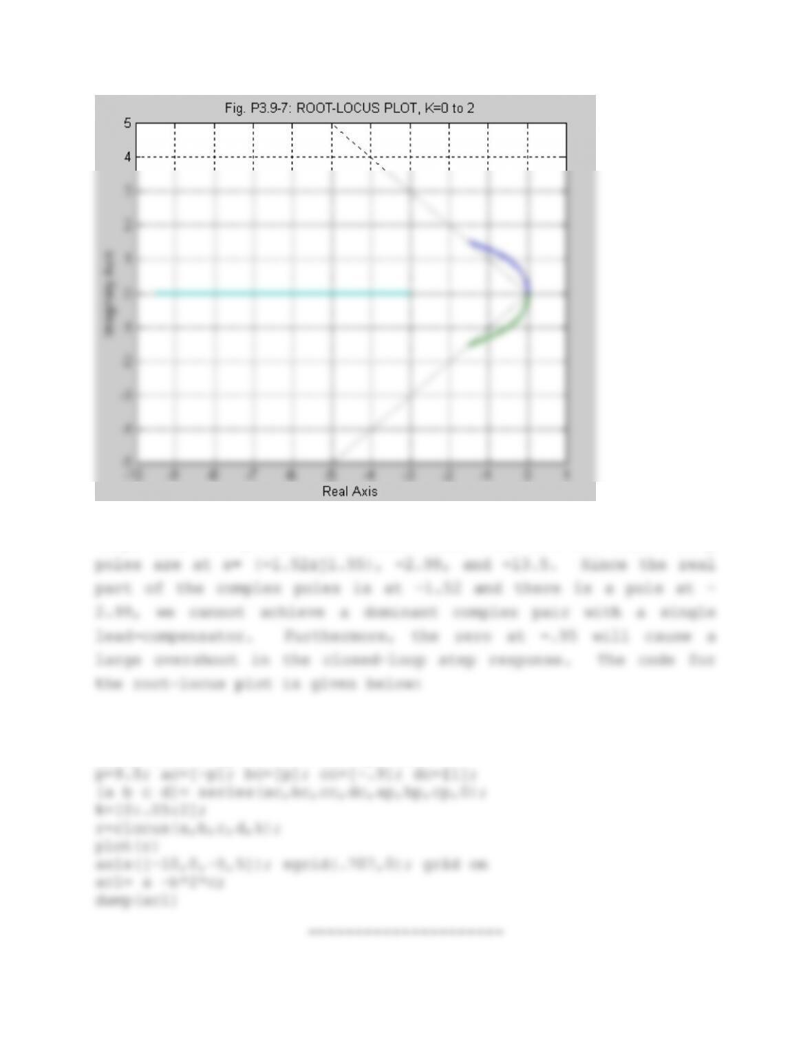
(z/p)=0.1, and p=9.5, this occurs when k=2, and the closed-loop
%Problem 3.9 -7
ap=[0 1 0; 0 0 0; 0 0 -10];
bp=[0 1 1]’; cp= [10 -1 1]; dp= [0];
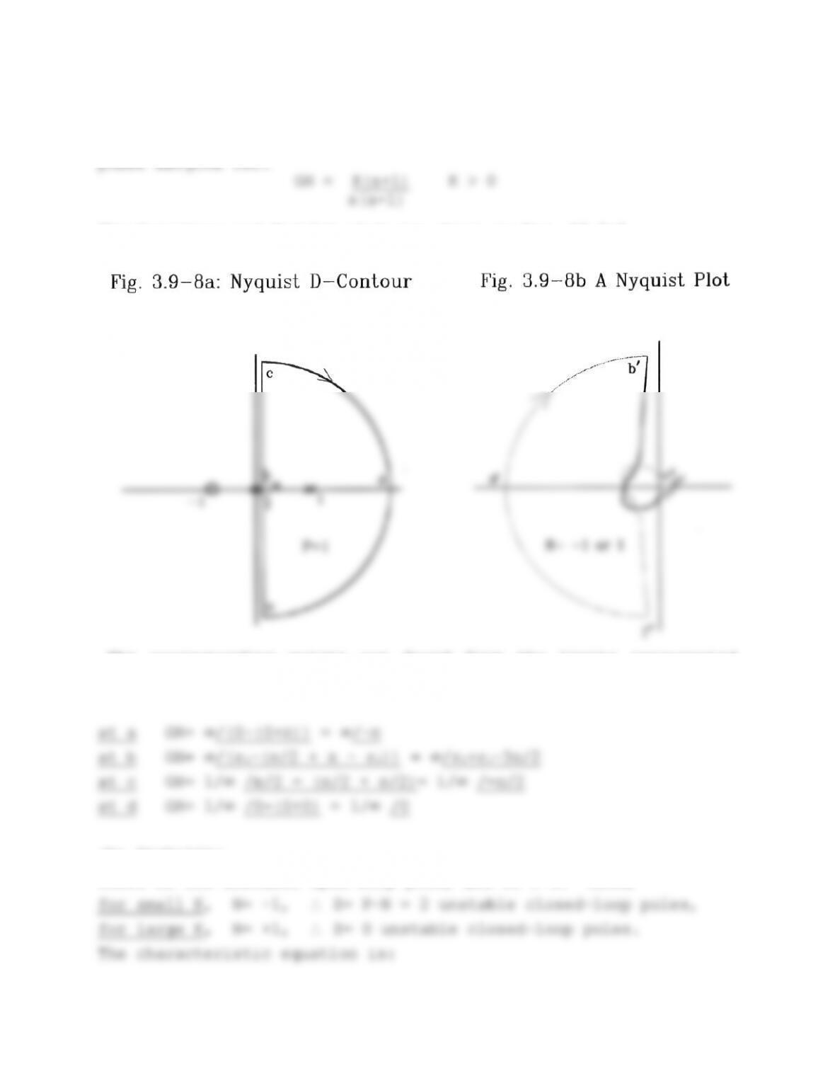
Problem 3.9-8: Nyquist plot, stability boundary, and gain and
phase margins for:
The D-contour and Nyquist plot are shown in Fig. P3.9-8.
The corresponding points are found from the limits represented
by:
(b) Stability
There is one unstable open-loop pole, and so P=1. Also,
which gives the stability boundary:
(c) Gain and Phase margins when K=2
The phase margin is found from:
From (1), the phase angle of the loop transfer function is given
Problem 3.9-9: Properties of a lead/lag transfer function.
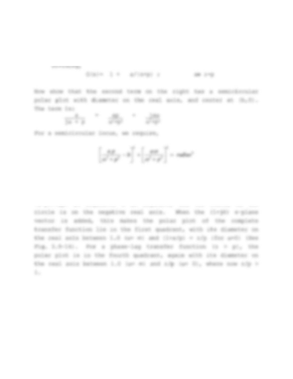
(a) Polar plot of G(s)= (s+z)/(s+p)
When the terms on the left are expanded, the dependence on
frequency is found to disappear if b= a/(2p), and then the radius
is also a/(2p). For a phase-lead (z < p) we find that a/(2p)=
(z-p)/(2p) is negative, b is negative, and the center of the
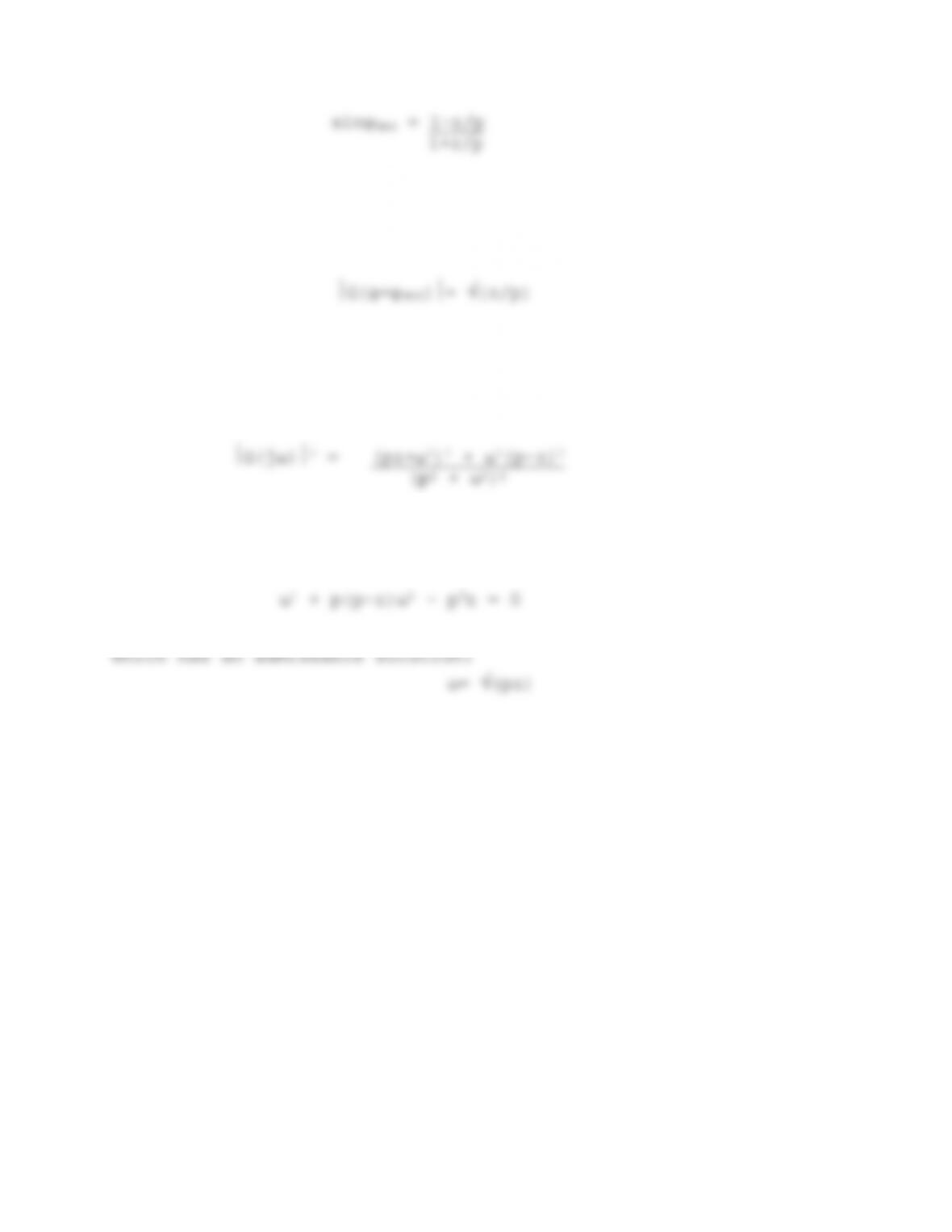
(b) Maximum lead or lag
Maximum lead or lag occurs when the radius vector of the
polar plot is tangential to the semicircle defined above (see Fig.
3.9-14). A radius of the semicircle to the point of contact makes
an angle of 90 deg. with the tangent. From this right-triangle we
find that,
and this formula applies to both the lag and lead cases. The
magnitude of the transfer function at the frequency of maximum
lead is easily found from one side of the triangle:
The frequency at which maximum lead or lag occurs can be found by
obtaining an expression for G, setting this equal to (z/p), and
solving for ω. Thus,
and expanding this, and putting G(jω)2= z/p, leads to:
and this applies to both the lead and lag cases.
(c) The polar plot for the phase-lag case is shown in Fig. P3.9-9
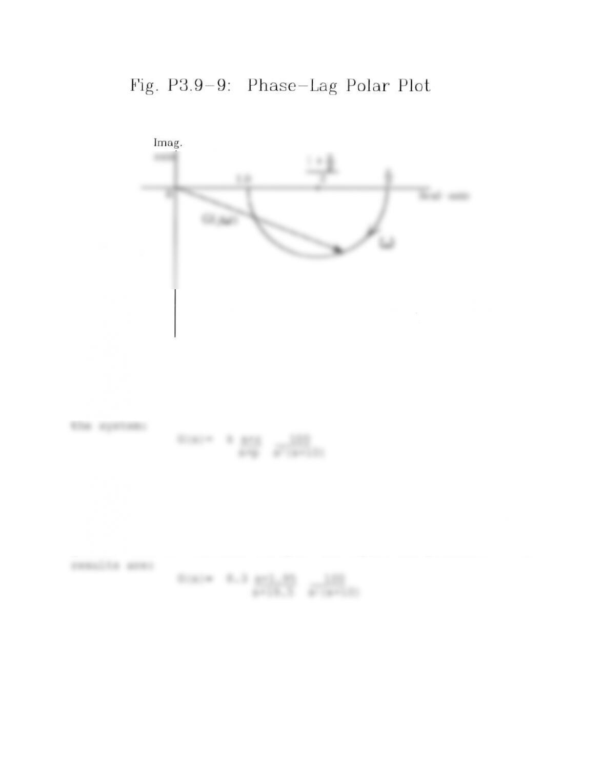
———————-
Problem 3.9-10: Design of a lead-compensator, with (p/z)=10, for
(a) Design for GM > 12dB and PM= 300
Fix the compensator pole-zero ratio and vary the pole
position to find the maximum phase margin; if the phase margin is
greater than 300 increase the gain and repeat the procedure. The
with a phase margin of 30.04 deg. and a gain margin of 13.80 dB.
The code is shown below.
(b) Design for GM > 12dB and PM= 450
Using the same procedure as in part (a), the results are:
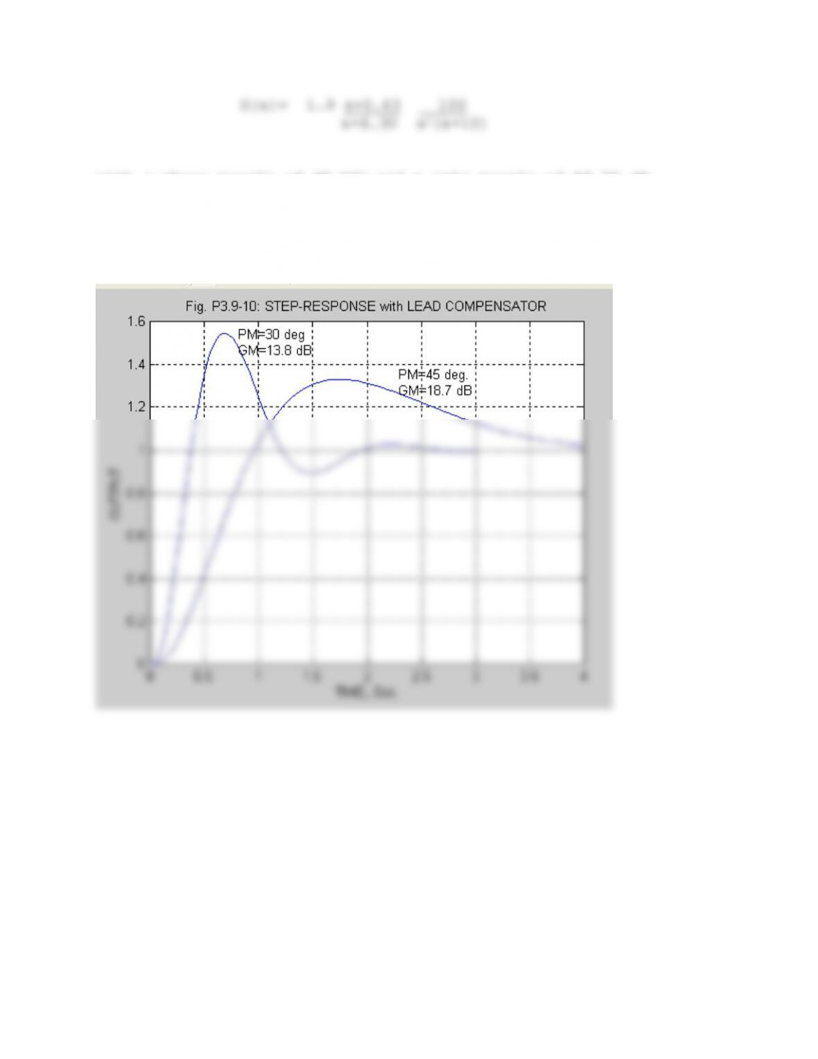
with a phase margin of 45.060 and a gain margin of 18.72 dB.
The step responses of these two designs are shown in Fig.
P3.9-10, it is clear that the design with the larger phase margin
is more heavily damped, has a smaller overshoot, and is slower.
%Problem 3.9-10. Design phase-lead compensator
if j==0
[mag,phase,omeg]=bode(a,gain*b,c,d); % Phase Margin plots
[gm,pm,wg,wp]=margin(mag,phase,omeg);
subplot(2,1,1),semilogx(omeg,20*log10(mag))