is about 0.9 ft. Therefore, the short-period involves essentially
only changes in alpha, theta, and pitch-rate, with very little
change in flight path angle as theta and alpha vary together.
————————-
Problem 3.8-2: Transport A/C; Throttle step-input time-history
simulation:
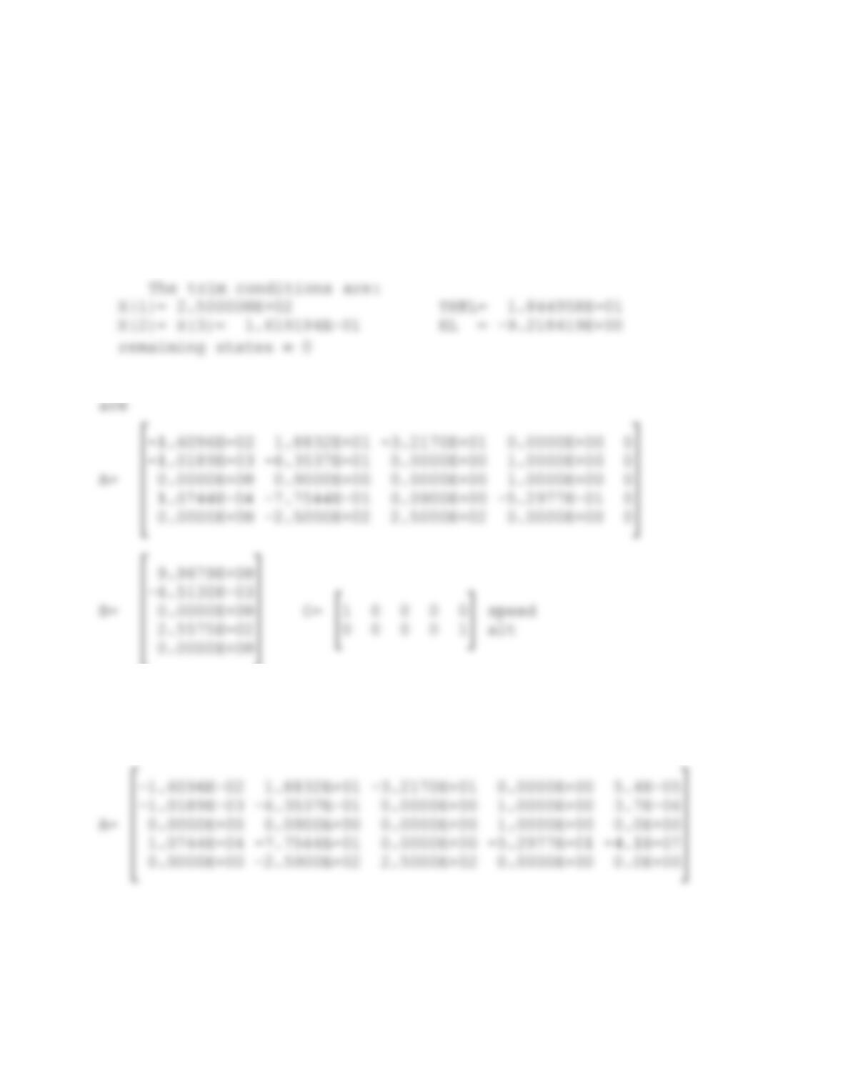
and the Jacobian matrices with no coupling from the altitude state
└ ┘
With altitude coupling included the B and C matrices are unchanged
and the A matrix becomes:
Speed and altitude responses can be obtained from these linear
models, and from the nonlinear aircraft model, with a throttle
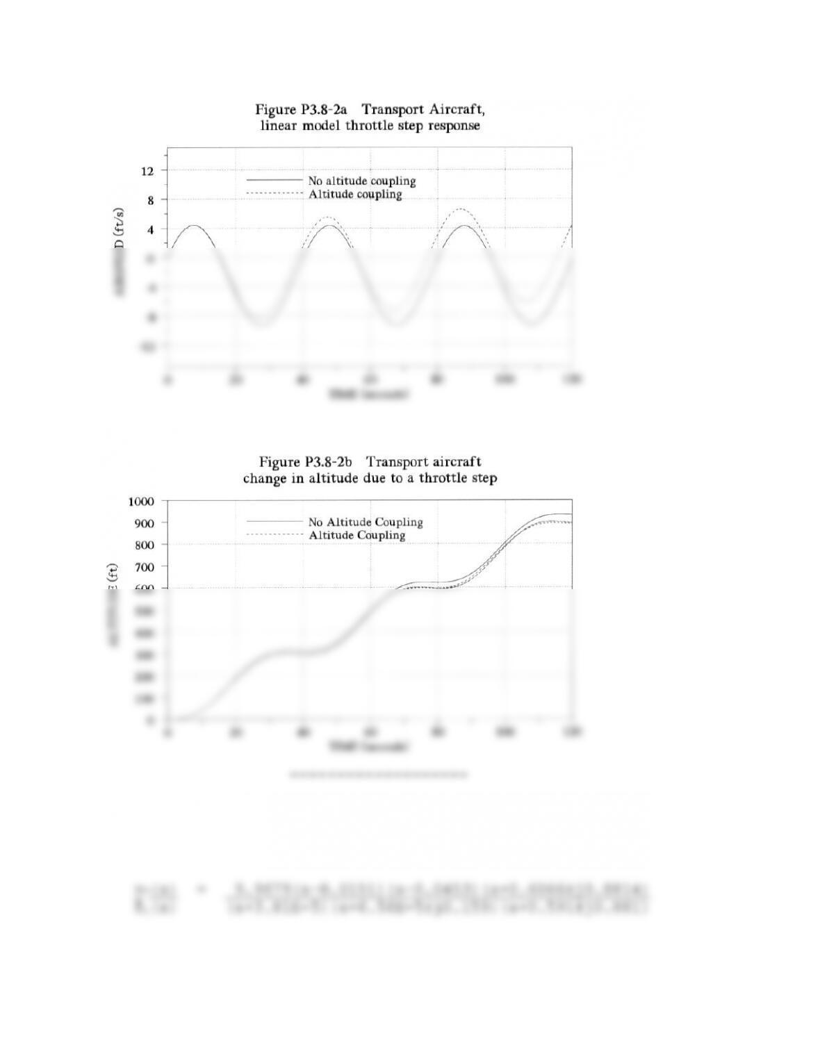
step input (of 0.1 units). The responses are shown in Figures
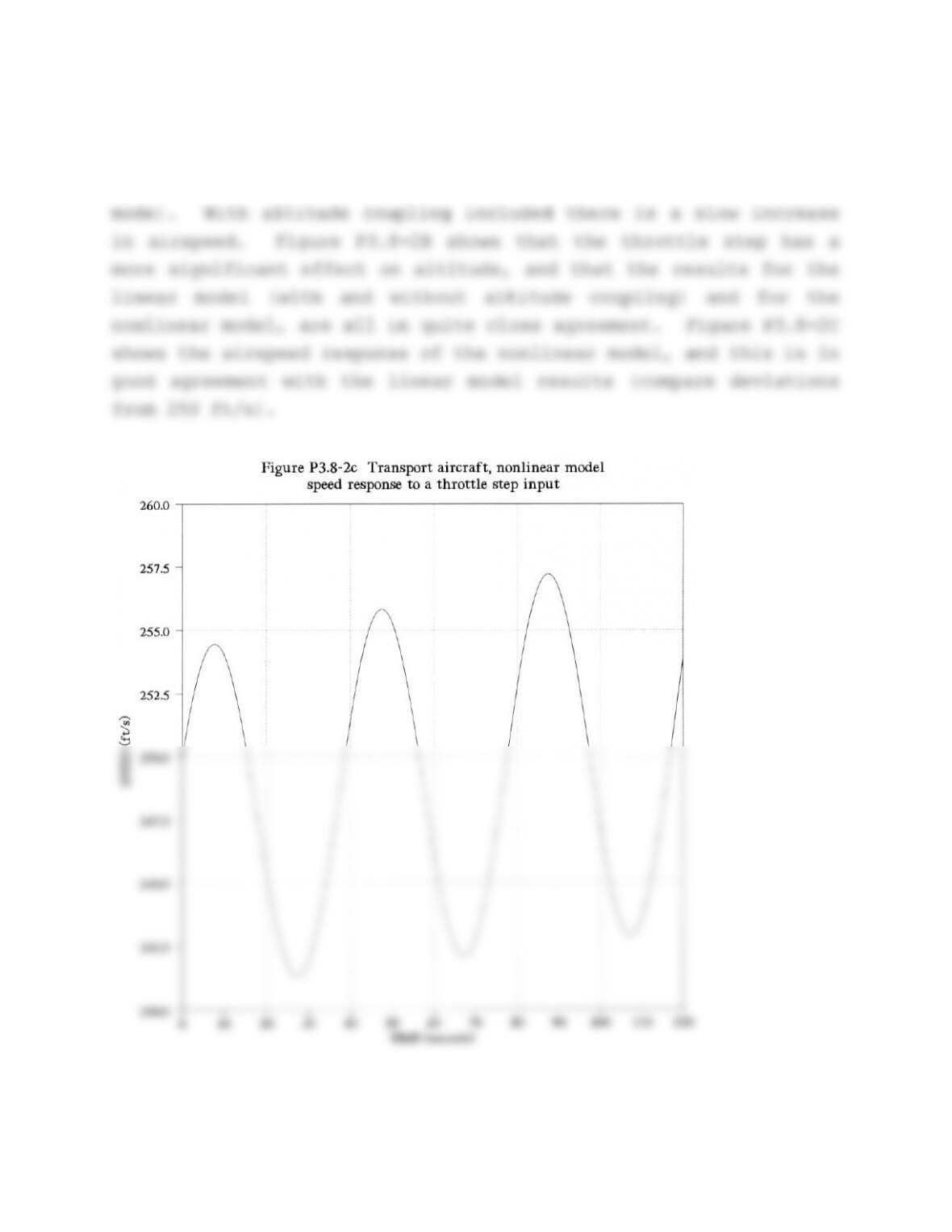
P3.8-2A through C. Figure P3.8-2A (linear model deviations from
trim speed) shows that, with no altitude coupling, a throttle step
does not increase the average airspeed (averaged over the phugoid
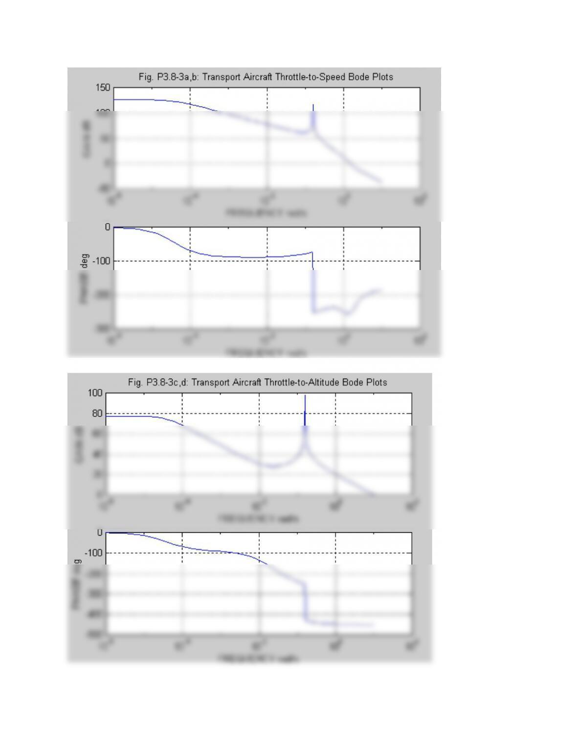
Problem 3.8-3: Bode plots for the transport-aircraft.
(a) Throttle-to-speed transfer function, VT(s)/δt(s).
The short-period poles are moderately well damped, and almost
coincident with a pair of zeros. Therefore, they will not be
visible in the Bode plots. This transfer function has two non-
minimum-phase (NMP) zeros. A sketch of the s-plane vectors for a
will fall at 20dB/dec. because the transfer-function rank (number
of poles – number of zeros) is 1.0. The Bode plots are shown in
Figs. P3.8-3A and B.
(b) Throttle-to-altitude transfer function, h(s)/δt(s).
This transfer function has no NMP zeros, and the short period

poles do not cancel out of the transfer function. The corner
frequency of the altitude pole is much lower than that of the
other poles and zeros, and so the asymptotic behavior of this
factor will be clearly visible in the Bode plots. The next corner
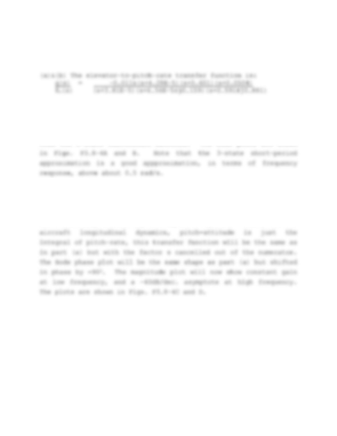
Problem 3.8-4: Transport-aircraft elevator transfer functions and
Bode plots using the same data as Problem 3.8-3.
and for easier interpretation of the phase, the sign of the
static-loop sensitivity will be ignored. A short-period
approximation was made by dropping the speed and altitude states
from the 5-state coefficient matrices. The Bode plots are shown
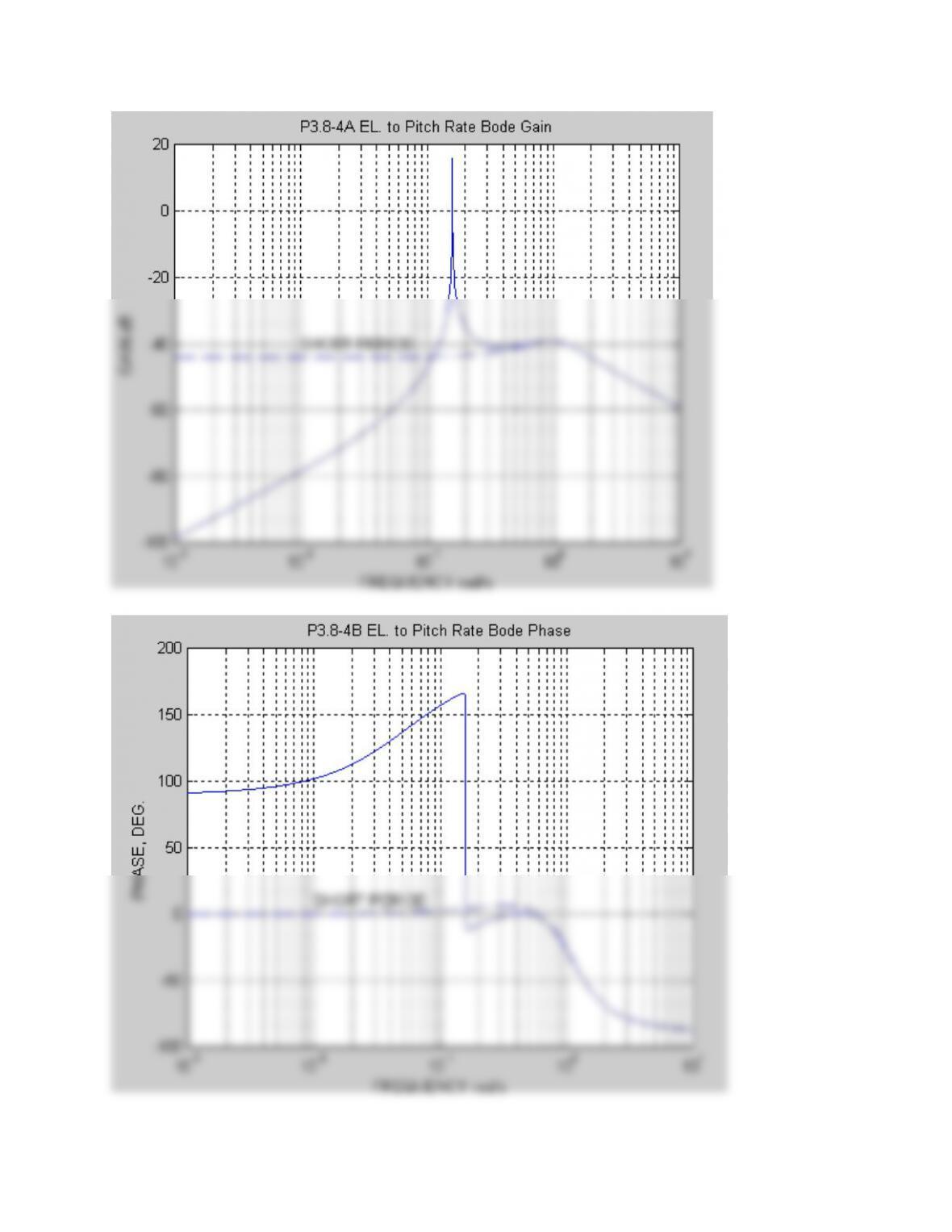
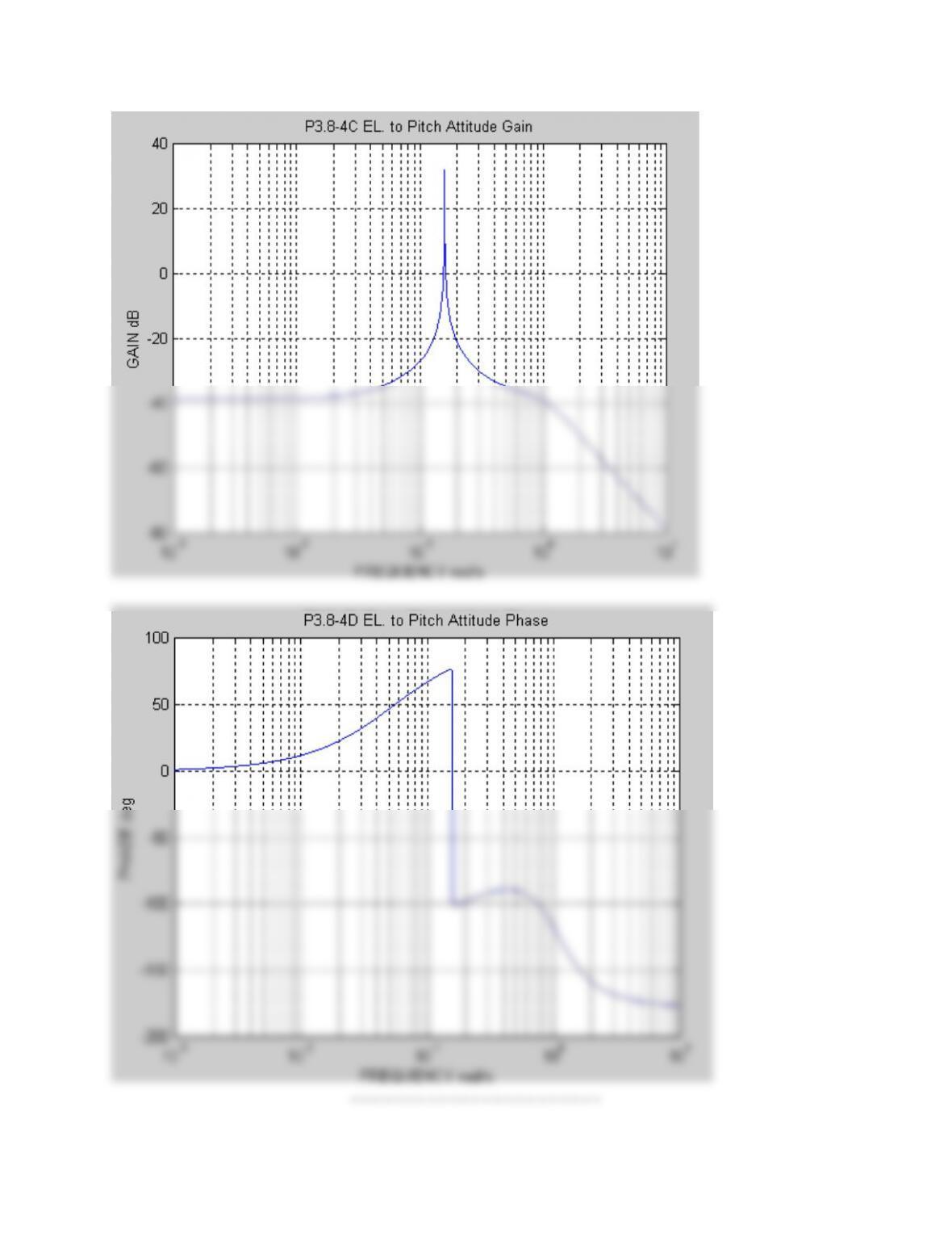
(c) Elevator-to-pitch-attitude transfer function
This transfer function is obtained from the 5-state coeffi-
cient matrices by choosing an appropriate C-matrix. The sign of
the static-loop-sensitivity will again be ignored. Since, for the
Problem 3.9-1: Control system steady-state error with a ramp
input.
(a) Hand calculation of s.s. error.
In the notation of Section 3.9, we have,
5.0
)(
0
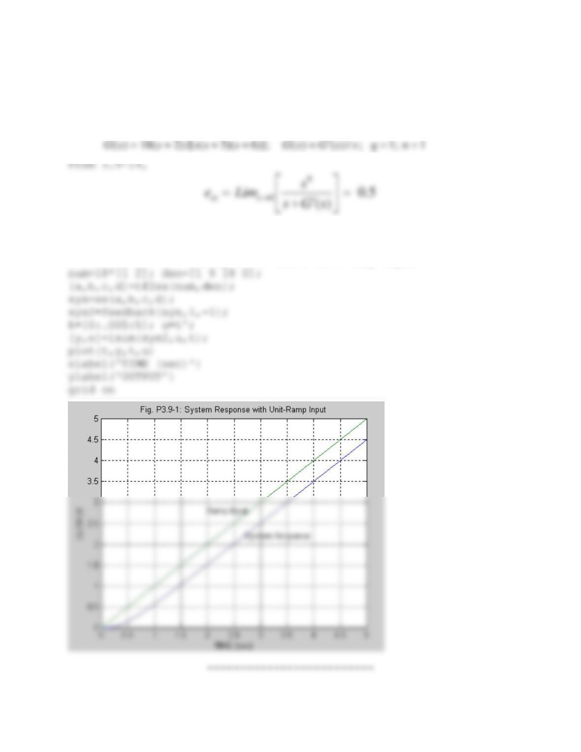
(b) The code for a simulation is given below. The resulting plot,
Fig. P3.9-1, also shows a steady-state error of 0.5 units.
% Problem 3.9-1. Steady-state error with ramp input
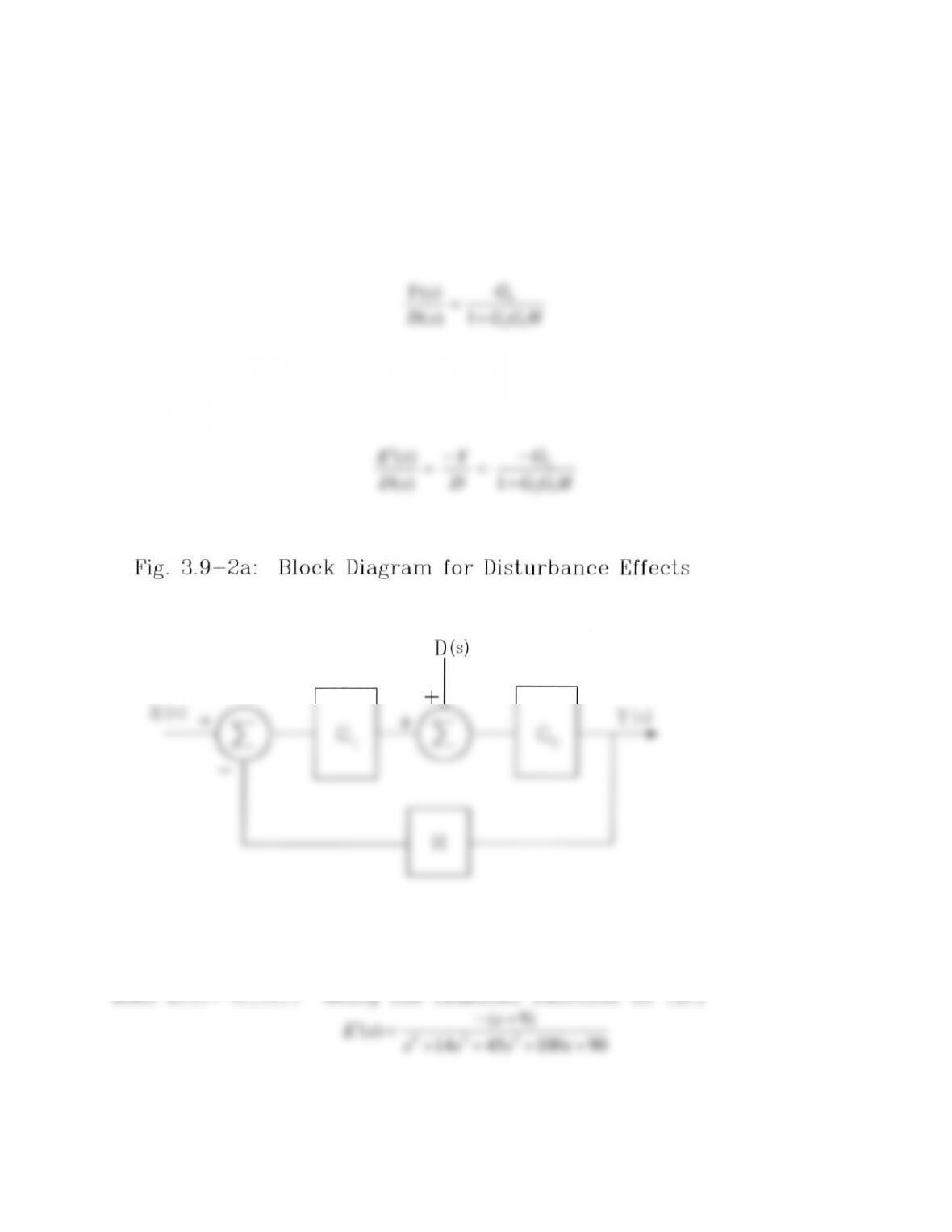
Problem 3.9-2: Closed-loop control with a disturbance.
(a) A block diagram of the system is shown in Fig. P3.9-2A, and
the transfer functions Y(s)/D(s) and E(s)/D(s), where E= R – Y,
must be found. Using the feedback formula, 3.9-4b, we obtain,
sD
12
1)(
Assuming linearity, the contribution,
E
, of D to the error comes
from -Y, and the transfer function is:
D
sD
12
1)(
(b) Given G1= 10/s; G2= 1/[s(s+5)]; H= 10(s+0.9)/(s+9); find )(te
ssss
and the s.s. error is ess= Lim(s->0)sF(s)= 0. A program to obtain the
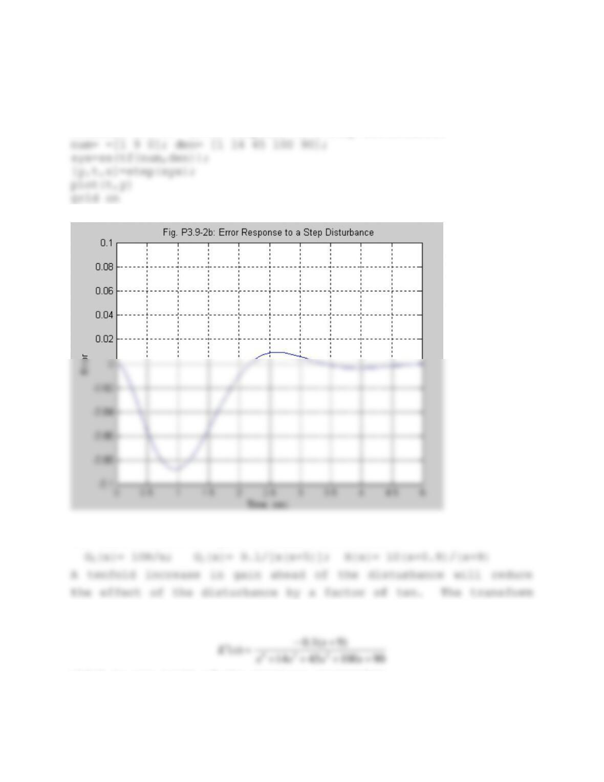
time response is given below, and the graph is shown in Fig. 3.9-
2B.
%PROBLEM 3.9-2. Error response to a step disturbance.
(c) Redistribute the gain to reduce the error:
of the step-response error is found to be:
ssss
which is one tenth of the previous expression.
———————-
Prob. 3.9-3:
(a) Determine k and z to achieve a closed-loop pole-pair with
ζ=1/5 and the highest possible error constant.
The system is type-II, so the relevant error constant is ka,
The root locus plot will have two complex branches leaving the
origin, and a branch from the pole to the zero along the real
axis. A root-locus sketch shows that placing the zero too far
left will reduce the maximum damping of the complex poles, while
placing the zero too far right will create a slow pole.
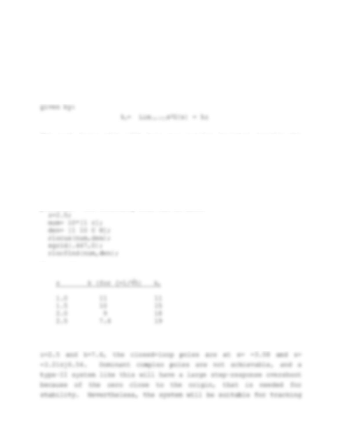
Therefore, we shall try a few different zero positions, adjusting
k for ζ=1/5 for the complex poles, and calculating ka for each
position. The following code can be used:
The results are:
ζ=1/5 is not achievable for values of z greater than 2.5. Using
with a small steady-state error when not subjected to step inputs.
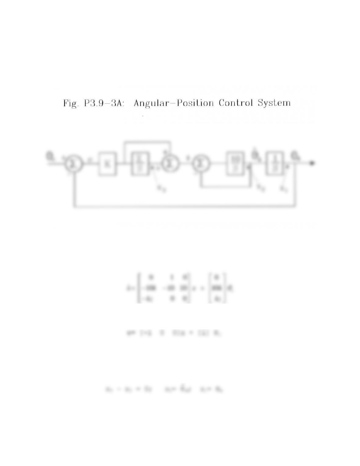
(b) Use as a tracking-antenna control system.
In Fig. P3.9-3A the system has been drawn as an angular
position control system with the set of state variables indicated.
The closed-loop state equations are:
kz
kz
00
The desired output variable is the error e= θc-x1 and so the C and
D matrices are given by:
An initial condition vector for steady-state tracking with e=0
(constant angular velocity tracking) is obtained by setting the
integrator inputs to zero, and then,
.
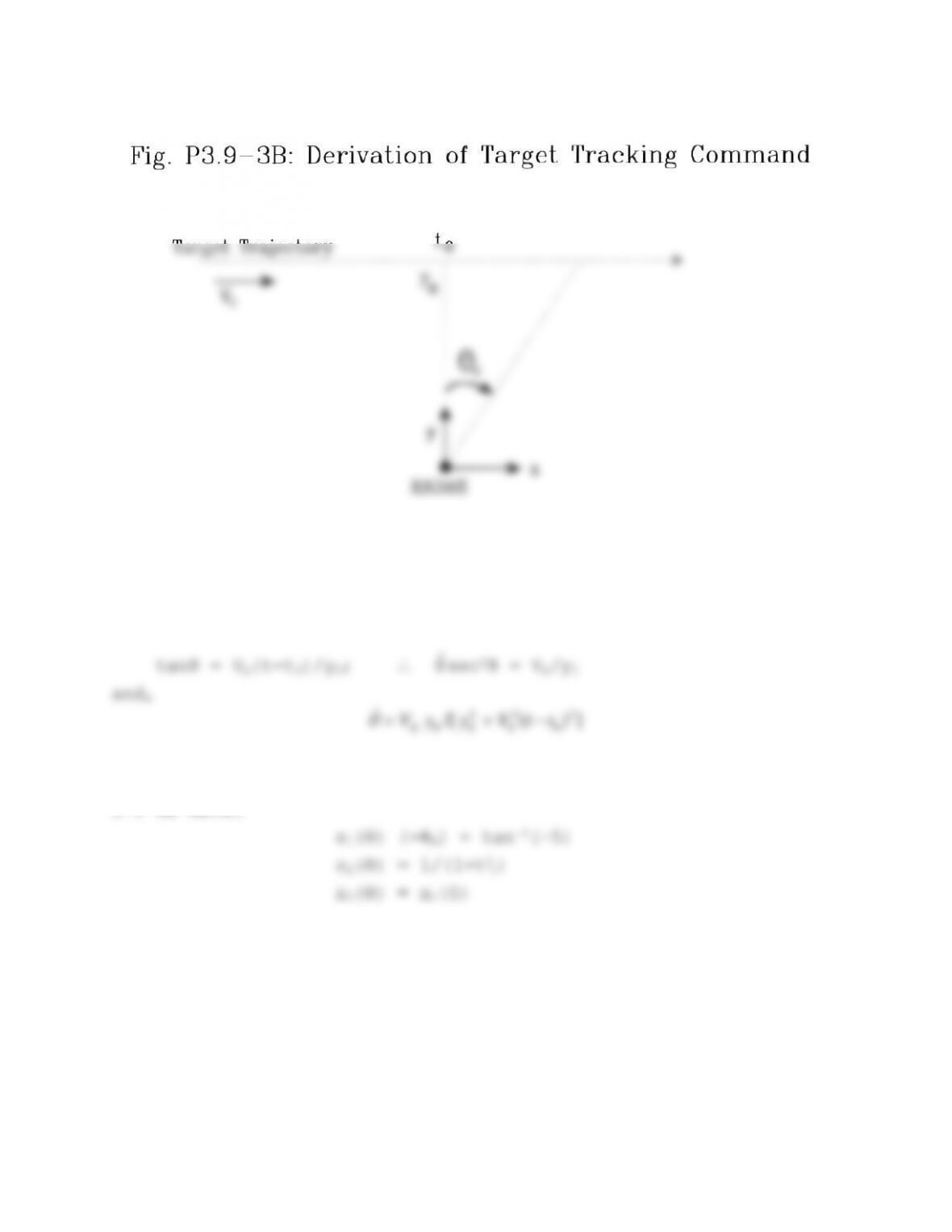
The angular command signal can be derived from the tracking
geometry shown in Fig. P3.9-3B, where t0 is the time of closest
approach:
])(/[ 2
0
0
00 ttVyyVX
The given initial conditions lead to t0= 5s and y0= 2000, and at
t=0 we have:
The simulation code is given below, and the plot of tracking error
is shown in Fig. P3.9-3C. Because the command contains derivatives
of all orders, the tracking error reaches large values (for radar
trackers) at the point of closest approach. Other techniques
(velocity feedforward) must be used to get acceptable performance.