Problem 3.4-2. Simulation of the Lorenz equations.
For second-order systems (e.g. Van der Pol, Example 3.4-1),
the possible autonomous (response to initial conditions) trajec-
tories in the two-dimensional phase space have been completely
classified. Particular trajectories can be identified by testing
the stability of the small-perturbation equations around “equ-
ilibrium” (or “singular”) points (where all the derivatives are s-
imultaneously zero, see Sections 2.6, 3.7), and by testing for
For the Lorenz equations, there are three possible singular
points:
but for r1 there is only one singular point, (0,0,0). The Lorenz
equations have reflection symmetry about the z-axis (reversing the
signs of both x and y yields an identical set of equations), and
this results in reflection symmetry of two of the singular points

The Jacobian matrix for linearizing the equations around a
singular point is:
When J is evaluated at the origin, the characteristic roots are
found from:
Therefore, the singular point at the origin is stable (three real,
negative roots) for 0<r1, and unstable (one positive real root)
for all r>1. For r>1 the two new singular points appear. These
points are reflections in the z-axis, and have the same stability
properties. Numerical calculation of the eigenvalues of J shows
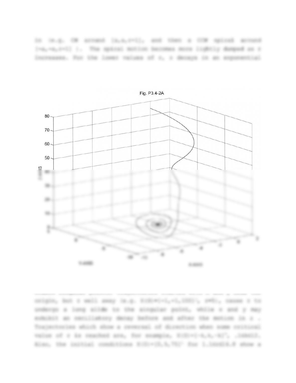
fashion and the x and y waveforms show a damped oscillatory decay.
Thus, a 3D phase portrait can appear as a helical motion tapering
toward the origin.
As r increases, in the range 1r<15, then, depending on the
initial conditions, a trajectory may go directly into a spiral
fashion to (r-1), and x and y show damped oscillatory decay. For
larger r, all three variables show lightly-damped oscillatory
decay.
For example, trajectories started near the origin (e.g. x(0)=
[±0.1,±0.1,±0.1]T, 2r13 ) will spiral directly to one of the
stable singular points; trajectories started with x and y near the
motion toward one singular point before landing on the other.
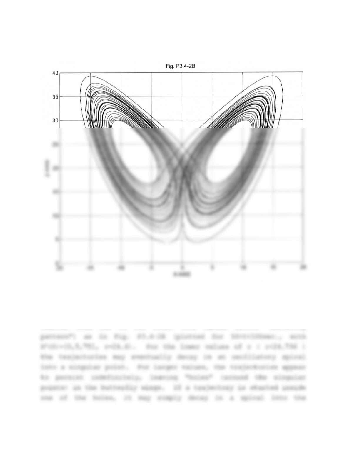
For r>16 the system can exhibit “chaotic” behavior
characterized by bursts of different frequency oscillation in the
waveforms, and phase portraits in which the trajectory circles
around both singular points and switches in a seemingly random
fashion from one to the other (the famous Lorenz “butterfly
singular point, or spiral outwards (r>24.736) to start the chaotic
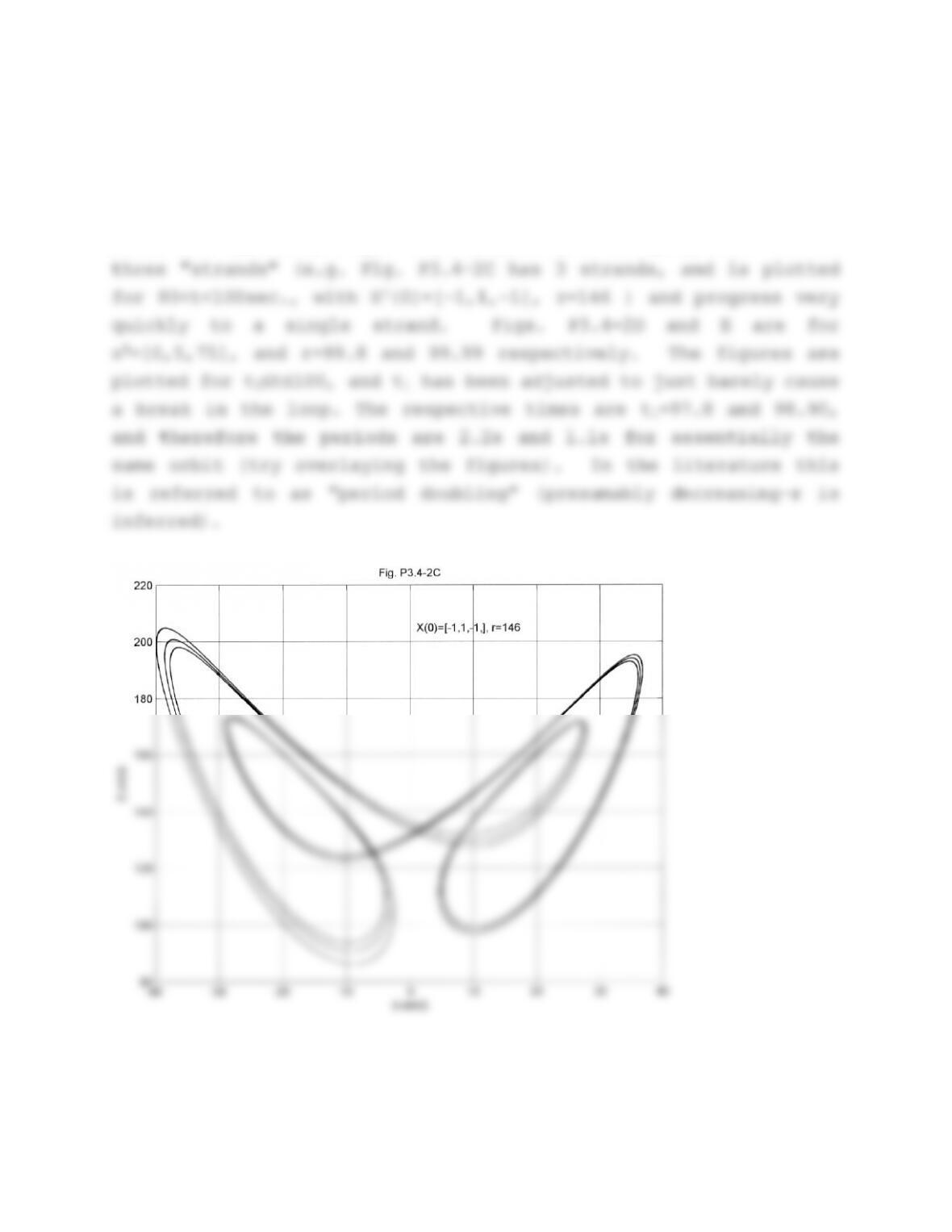
behavior. The range of r in which the behavior is chaotic is
broken up by small intervals of r in which the asymptotic
trajectory is a periodic orbit around both singular points. The
intervals typically begin with trajectories clumping into two or
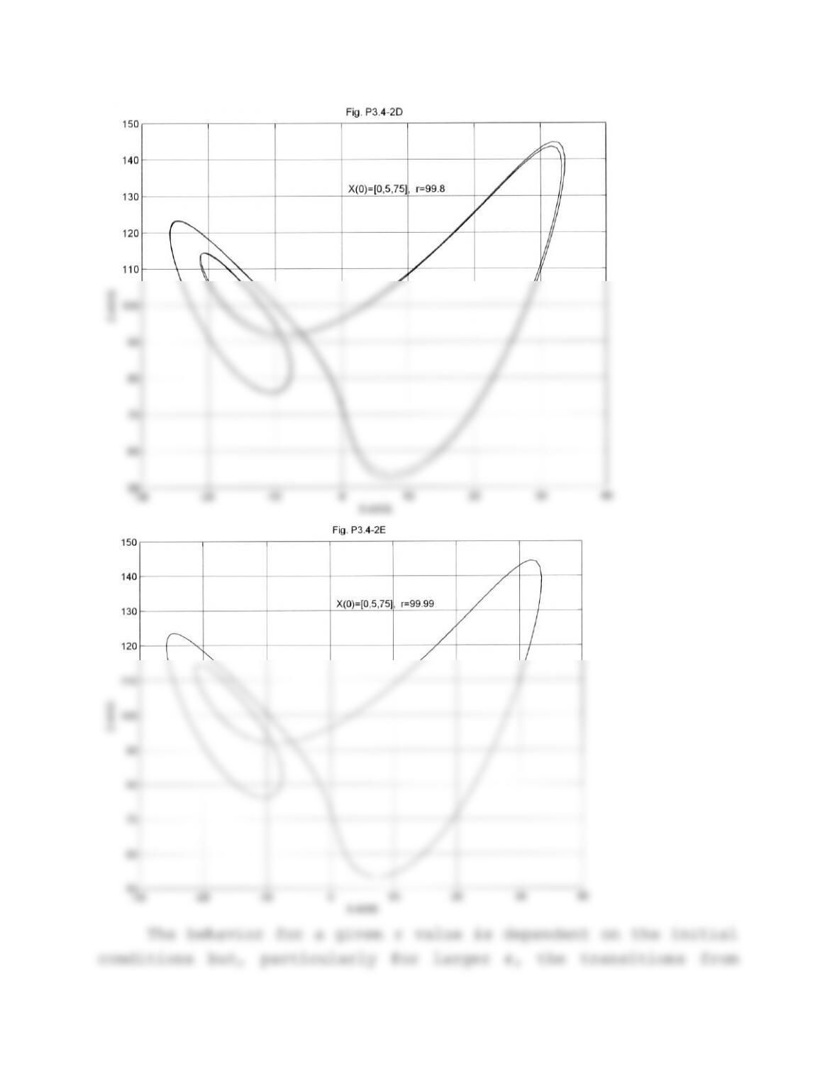
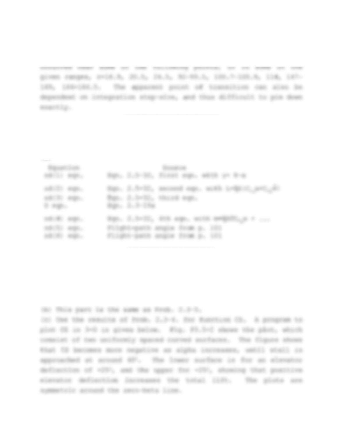
chaotic to periodic or vice-versa occur at about the same point.
For the three sets of initial conditions above, transitions
————————
Problem 3.5-1: Construct and verify the transport aircraft model.
Parts (a) and (b) are self-checking.
(c)
———————-
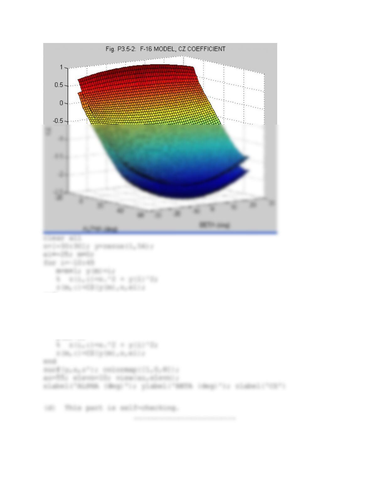
Problem 3.5-2: Construct and verify the F-16 model.
(a) See Probs. 2.3-4 through 2.3-6 for details of constructing the
F-16 aerodynamic tables with linear interpolation.
end
surf(y,x,z’); hold on; colormap([0,0,0]);
el=25; m=0;
for i=-10:45
m=m+1;
y(m)=i;
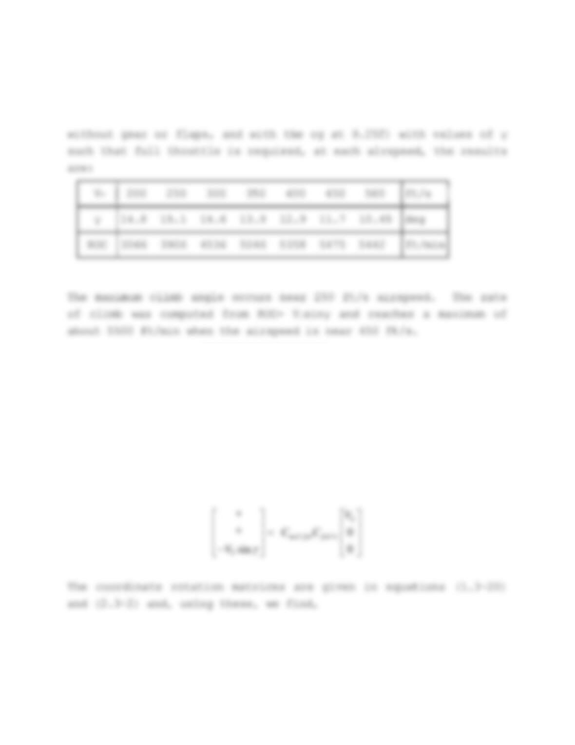
Problem 3.6-1: Trim and rate-of-climb of the transport aircraft.
(a) This part is self-checking.
(b) If the transport aircraft model is trimmed (at sea level,
_) with values of γ
——————-
Problem 3.6-2: F-16 model trim.
This problem is self-checking.
———-———–
Problem 3.6-3: Derivation of flight-path constraints.
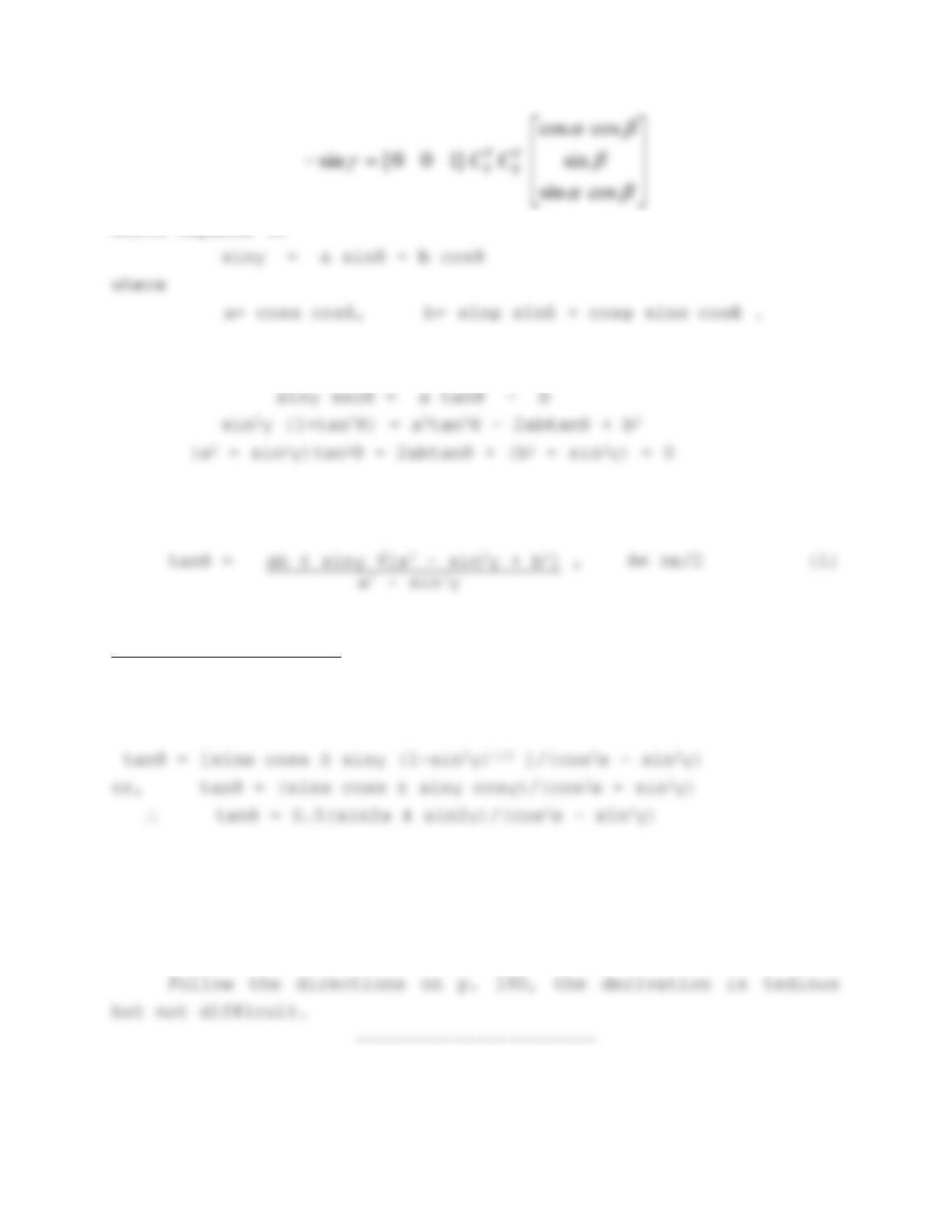
3.6-3(a) Derivation of the ROC constraint, Eqn. 3.6-3:
Start from Equation (3.6-1):
0
sin
//
wfrdfrdned
T
V
cossin
sin
coscos
]100[sin TT CC
which expands to
Now assume θ ±π/2, divide through by cosθ, and solve for θ
Solving the quadratic for θ gives
a
choice of sign in (1)
When β=0 and φ=0, then a= cosα and b= sinα, and the equation for
tanθ becomes
For small angles this approximates θ = α ± γ, which we know
should have a positive sign; therefore we use the + sign in (1).
3.6-3(b) Derivation of the turn-coord. constraint, Eqn. 3.6-5:
Problem 3.6-4: Trimming for a prescribed angle of attack.
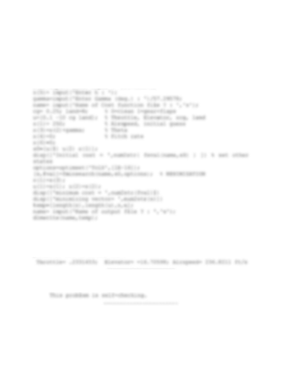
A modification of the trim program given in the text, to trim
the aircraft for a specified angle of attack, is shown below.
% TRIM.m
clear all
global x u gamma
x(2)=input(‘Enter Alpha : ‘)/57.29578;
(b) Trim for α=150 at 10,000 ft.
The results given by the above program, with the TolX
parameter set to 1E-16, are:
———-———–
Problem 3.6-5: Duplicate the results of Exs. 3.6-3 and 3.6-4.
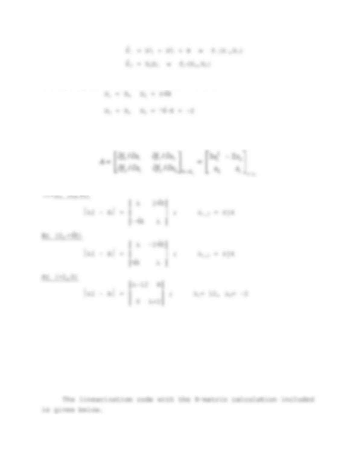
Prob. 3.7-1: Small-perturbation analysis of nonlin. state eqns.:
.
(a) By inspection, the singular points are:
(b) Jacobian matrix:
e
XX
exx
xx
xfxf
xfxf
XX
12
2
2
1
2212
2111 23
//
//
In the first and second cases we might expect a constant amplitude
oscillation around the singular point, and in the second case we
expect the trajectory to depart from the singular point because of
the unstable mode e12t.
———-———–
Prob. 3.7-2: Linearization algorithm for B-matrix, confirm
Ex.3.7-1
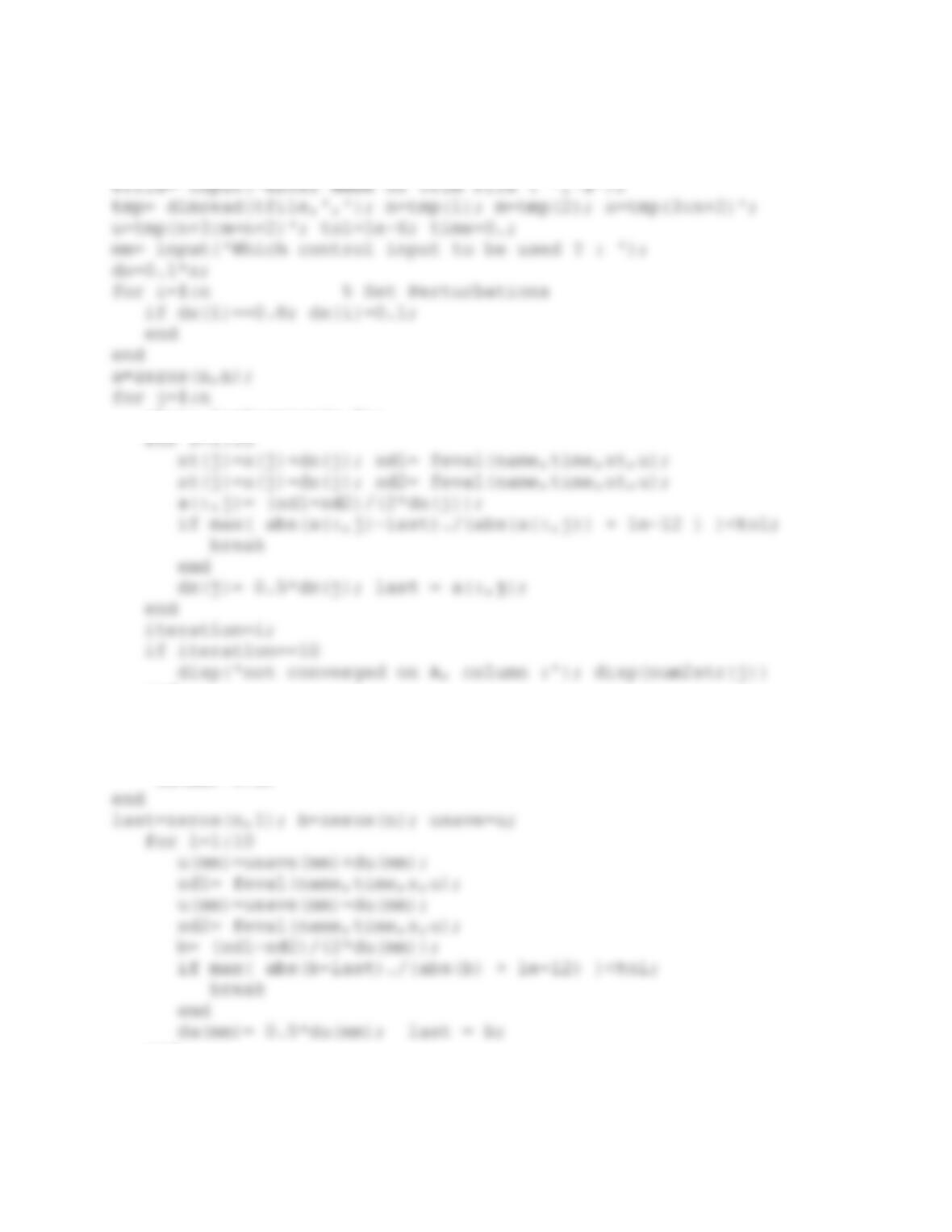
(a)% File LINZE.m
clear all
name = input(‘Enter Name of State Eqns. File :’,’s’);
xt=x; last=zeros(n,1);
end
end
du=0.1*u; % Set Perturbations for B
if du(mm)==0.0;
du(mm)=0.1;
end
iteration=i;
if iteration==10
(b) This algorithm yields the same B-matrix as in Ex. 3.7-1 (most
elements agree to five digits). Note that if a hard limit has
been placed on the throttle input, it should be disabled for
linearization.
———————-
Prob. 3.7-3: Coefficient matrices from stability derivatives.
The following program reads the flight conditions from a
data-file produced by the trim program. These are used with the
stability derivatives of the transport aircraft model to calculate
% Program to solve Problem 3.7-3. 20 April 2004
MASS=5.0E3; IYY=4.1E6;
S=2170; CBAR=17.5; G=32.17; XCGR=0.25; XCG=0.25;
TSTAT=6.0E4; DTDV= -38;
RTOD=180/pi;

CD= CD0 + CDCLSQ*CL^2 + CDELSQ*ELDEG^2;
CM= CM0 + CMA*ALPHA + CMDE*ELDEG + CL*DUM; % Aerodynamic only
CDA= CDCLSQ*2*CL*CLA;
SGAM= sin(GAMMA);
CGAM= cos(GAMMA);
SALP= sin(ALPHA);
CALP= cos(ALPHA);
DTDTH= (TSTAT + DTDV*VT);
———————–
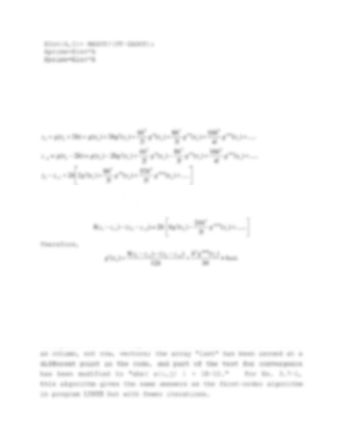
Problem 3.7-4: (a) Derive the third-order linearization algorithm
(Eqn. 3.7-4) and (b) evaluate its performance.
(a) Using the same notation as Section 3.7, we have,
…..)(
!5
32
)(
!3
8
)(22
!4
!3
!2
43
22
2
eee
eeeeee
vg
h
vg
h
vghzz
Now combine (z1-z-1) and (z2-z-2) to eliminate the g
term:
24
4
h
The first term on the right gives an approximation to the deriva-
tive of g with respect to v that includes Taylor-series terms
through h3.
(b) Linearization program
The program LINZE in the textbook has been modified to
incorporate the above algorithm. Also, x and u have been treated
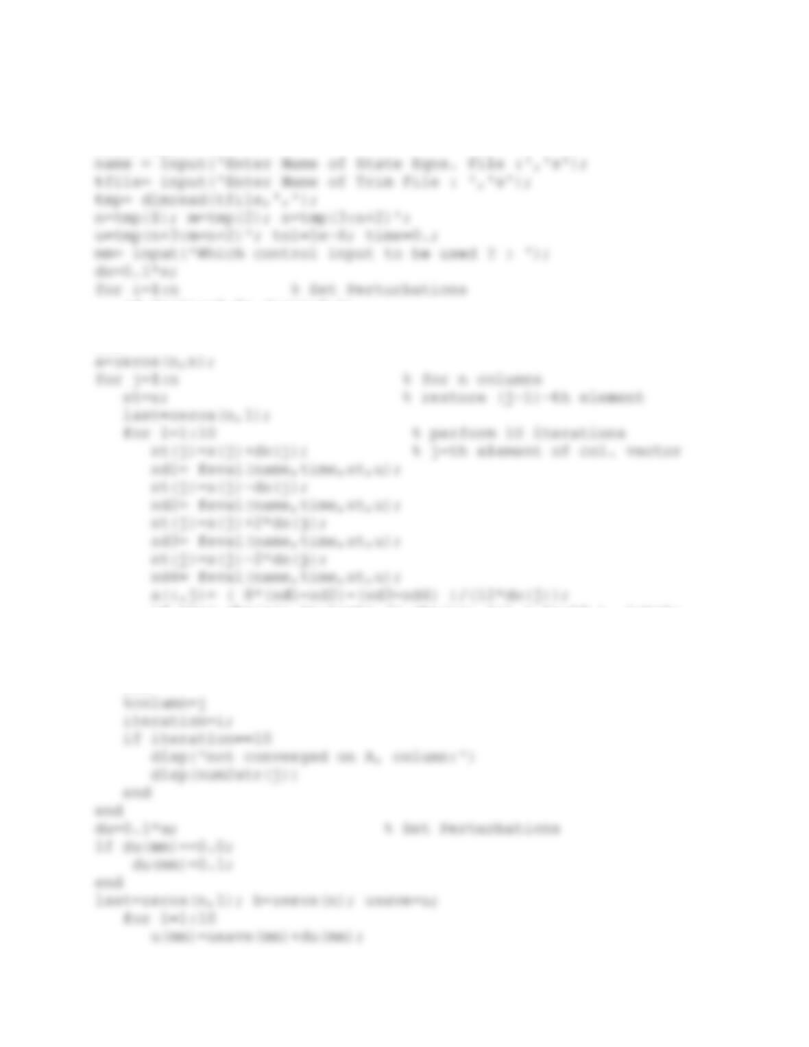
% File LINZE2.m
clear all
if dx(i)==0.0; dx(i)=0.1;
end
end
if max( abs(a(:,j)-last)./( abs(a(:,j)) + 1e-12 ) )<tol;
break
end
dx(j)= 0.5*dx(j); last = a(:,j);
end
iteration=i;
if iteration==10
disp(‘not converged on B’)
end
———————-
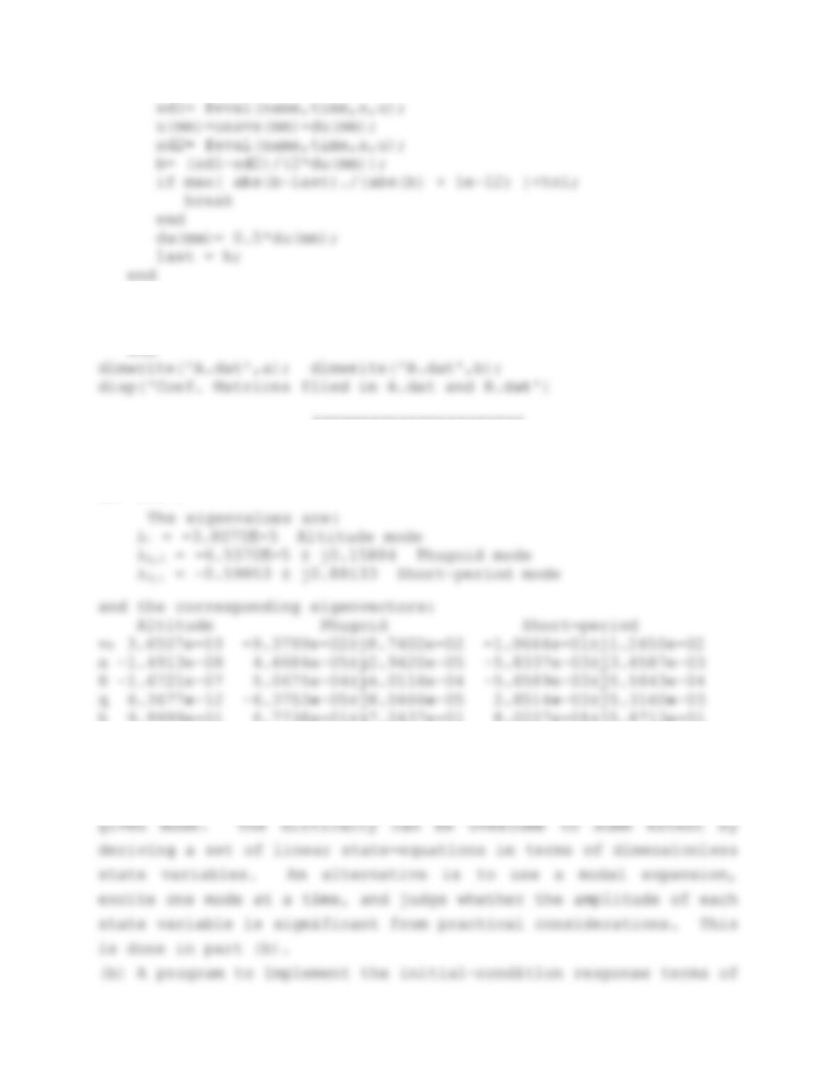
Problem 3.8-1: (a) Find the eigenvalues and eigenvectors of A in
Ex. 3.8-5
h 9.9999e-01 6.7738e-01±j7.2437e-01 8.0227e-01±j5.8713e-01
Because the eigenvectors are not dimensionless, it is difficult to
determine how significantly each state variable participates in a
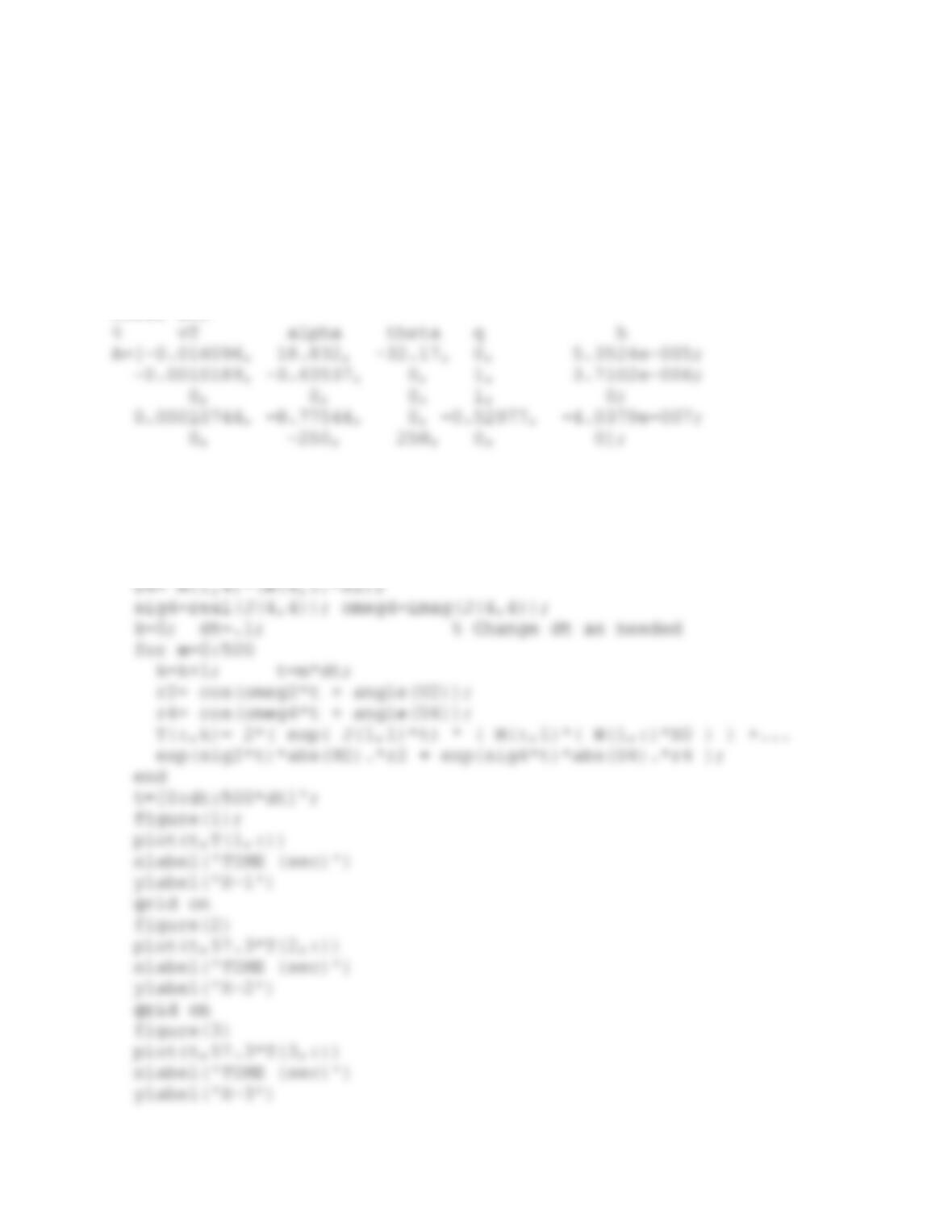
the modal expansion (3.2-15) is given below. A complex initial
condition vector is necessary to excite a complex mode but the
results are a set of real waveforms. To evaluate the real
response, complex conjugate pairs of terms are combined into real
terms.
% Problem 3.8-1; Modal expansion, Example 3.8-5 dynamics
clear all
[M,J]=eig(A,’nobalance’); % A*M = M*J
W=inv(M); % Inverse of Modal Matrix
X0=M(:,2); % Initial condition = eigenvector
U2= M(:,2)*(W(2,:)*X0);
sig2=real(J(2,2)); omeg2=imag(J(2,2));
The matrix of eigenvalues (“J” in the code) shows that the
first eigenvalue is for the altitude mode, the second and third
for the phugoid mode, and fourth and fifth for the short period.
The eigenvectors are computed in the same order, so that v1
corresponds to the altitude mode, and so on. When x0=v1 and
0t5E4, all of the states show exponential changes. The altitude