CHAPTER 3
Problem 3.2-1: State equations for the system in Fig. P3.2-1.
The extensions of the two springs and velocities of the two
masses determine the stored energy, and none of these variables
can be related to some linear combination of the input and the
other three variables alone. Therefore four state variables are
needed to specify the stored energy. The most straightforward
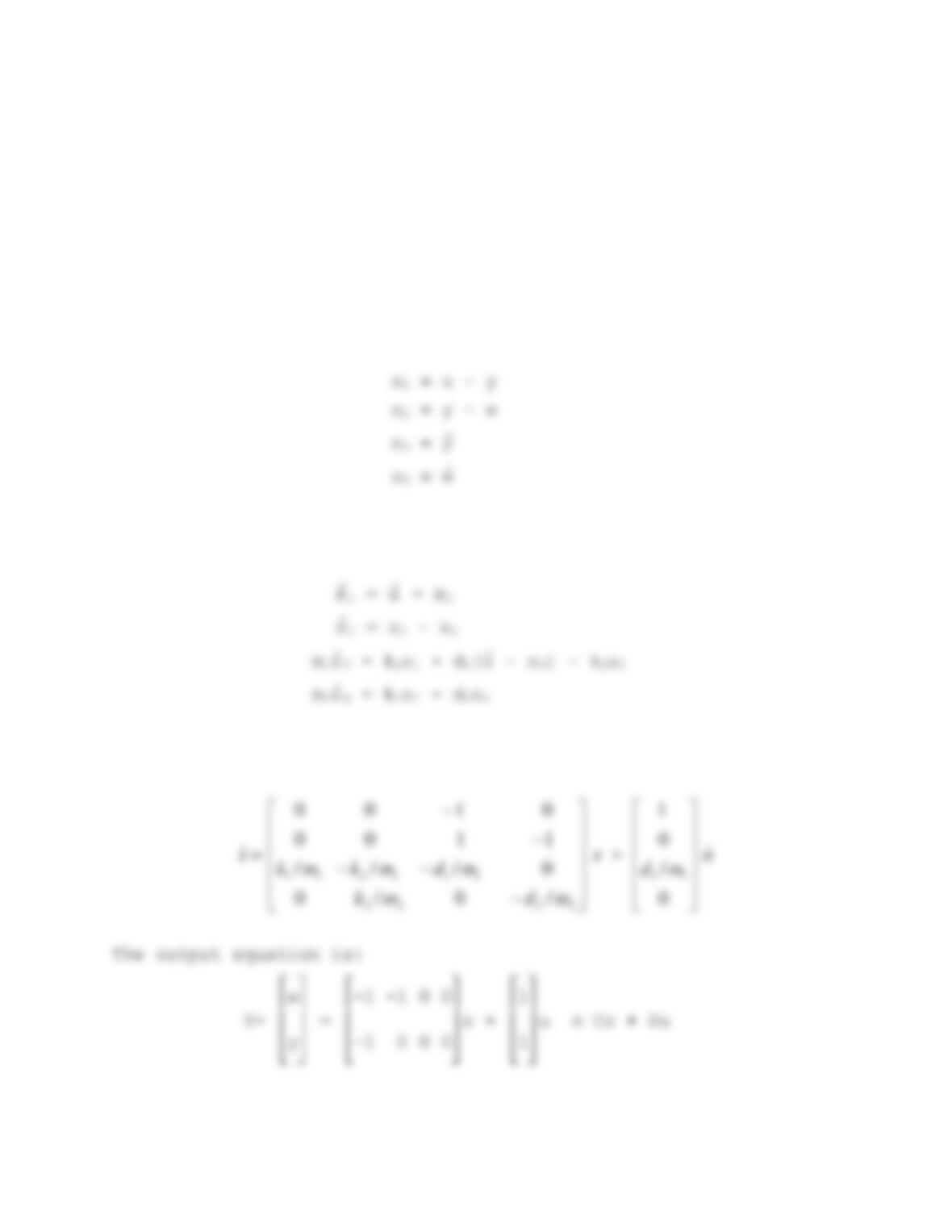
choice of state variables is:
x
4 w
By inspection of the diagram, the state equations are:
.
. – x3
Now arrange these in the matrix form x
.= Ax + B1u
.,
0
1
1100
0100
Only the state equation has a u
. term, and so the transformation
given in the text can be used successfully to obtain a pair of
equations with no derivative of the input. The new state equation
is:
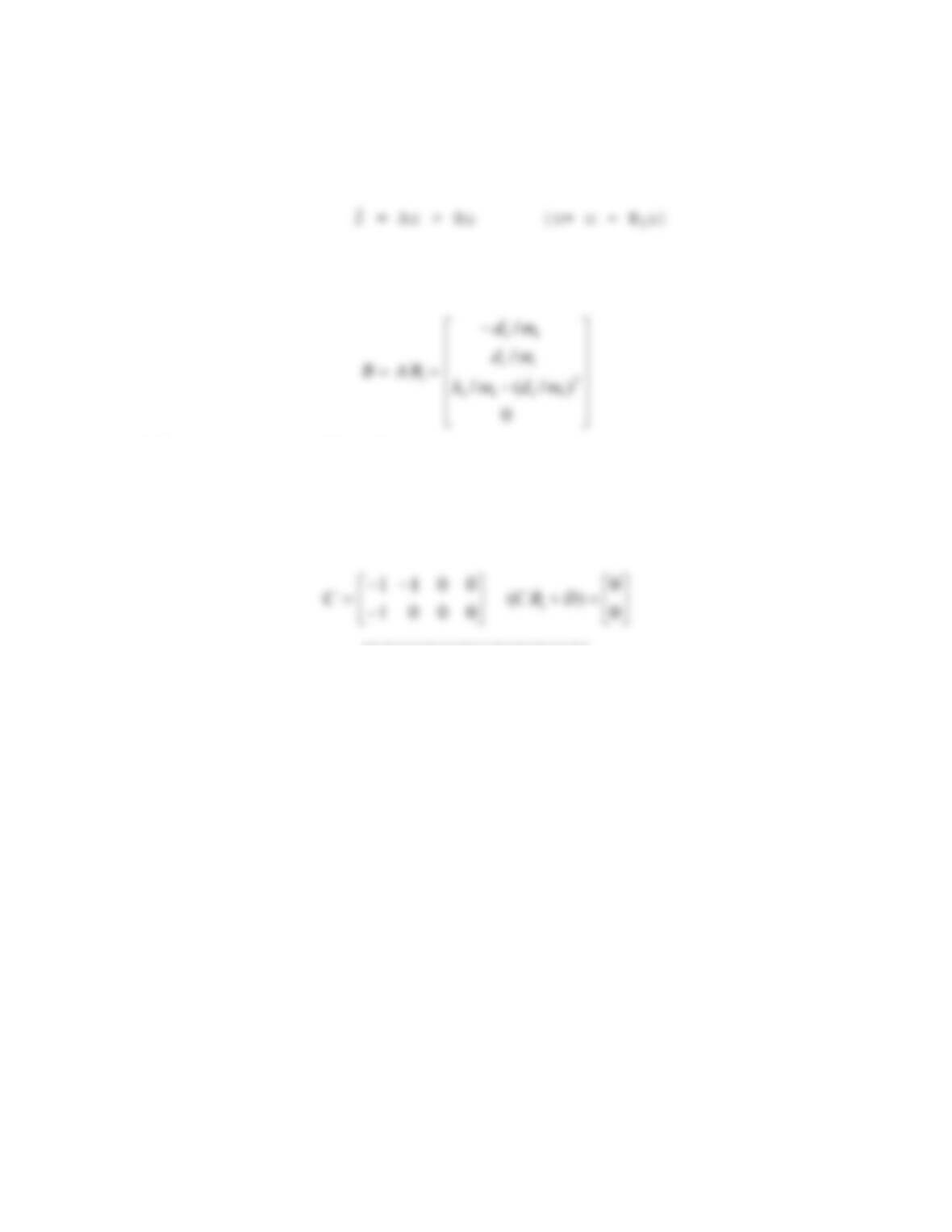
z
. = Az + Bu (z= x – B1u)
where A is given above, and B is:
0
)/(/
/
/
2
1111
11
11
1mdmk
md
md
and the output equation is:
Y = Cz + (CB1 + D)u
where the coefficient matrices are:
0001
———-———–
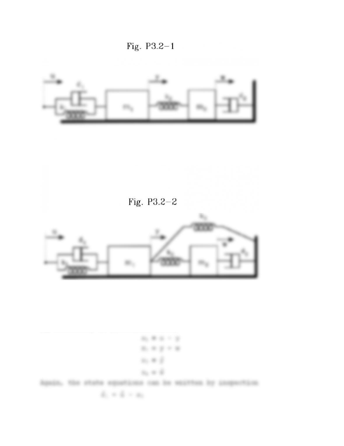
Problem 3.2-2: State Equations for Problem 3.2-1 with an added
spring, k3.
Compression of k3 is determined by u and the compression of
k1, therefore, as in Problem 3.2-1,
x
1 = u
.
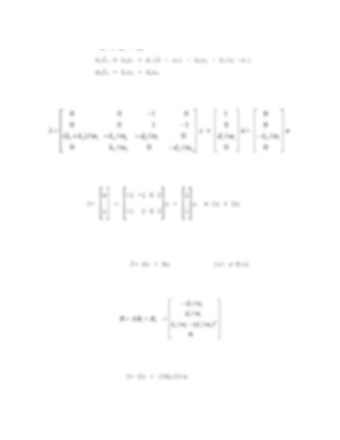
The matrix form is now x
.= Ax + B1u
. + B0u, or,
u
mk
md
mdmk
mdmkmkk
0
/
0
/
/0/0
0///)(
13
11
2222
1112131
The output equation is the same as Problem 3.2-1:
and contains no derivative term. Therefore, the transformation
given in the text can be used again. The new state equation is:
where A is given above and B is:
0
)/(/
2
1111
01 mdmk
which is the same as Prob. 3.2-1. The new output equation is:
0
0001
0011
which is also the same as Prob. 3.2-1
———-———–
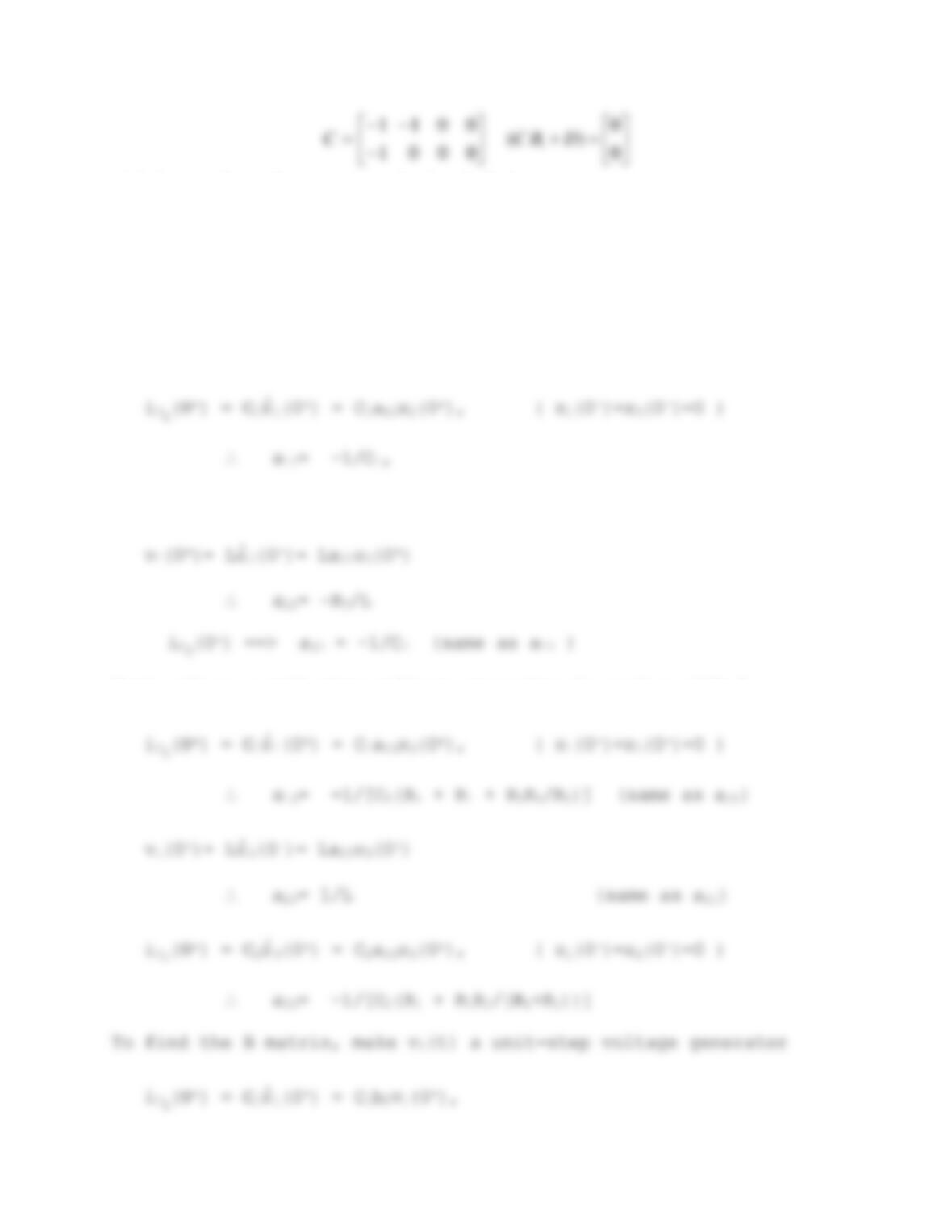
Problem 3.2-3: State equations for the Bridged-T circuit.
The first column of the A-matrix is given in the textbook; to
find the second column, put a unit-step current generator in
parallel with L, so that:
.
(the short-circuit capacitors see 100% of the current)
Next, place a unit-step voltage generator in series with C2
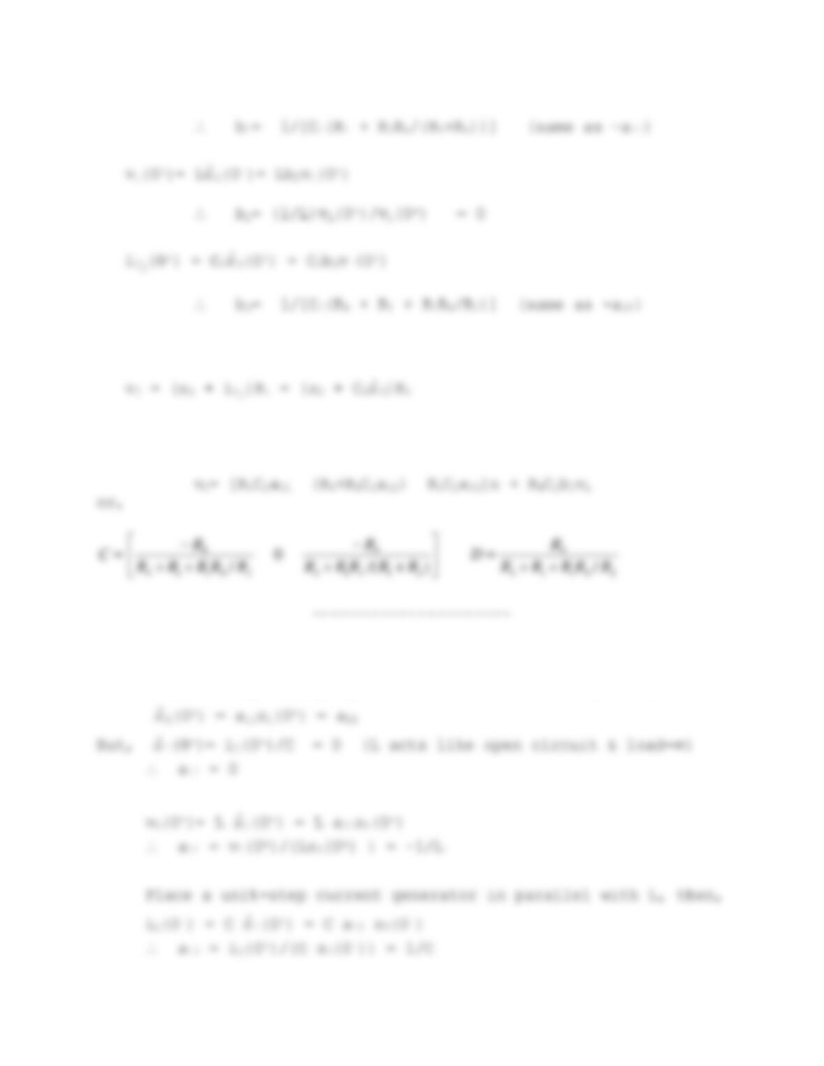
The output equation can be found as follows:
.
from which we find that,
Problem 3.2-4: State equations for the quadratic lag, Fig. P3.2-4
Place a step-voltage generator in series with C, then,
.
———————–
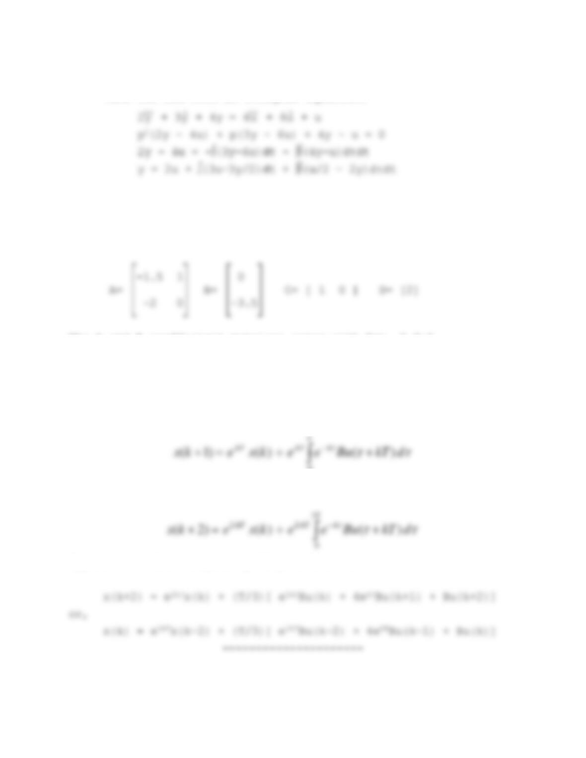
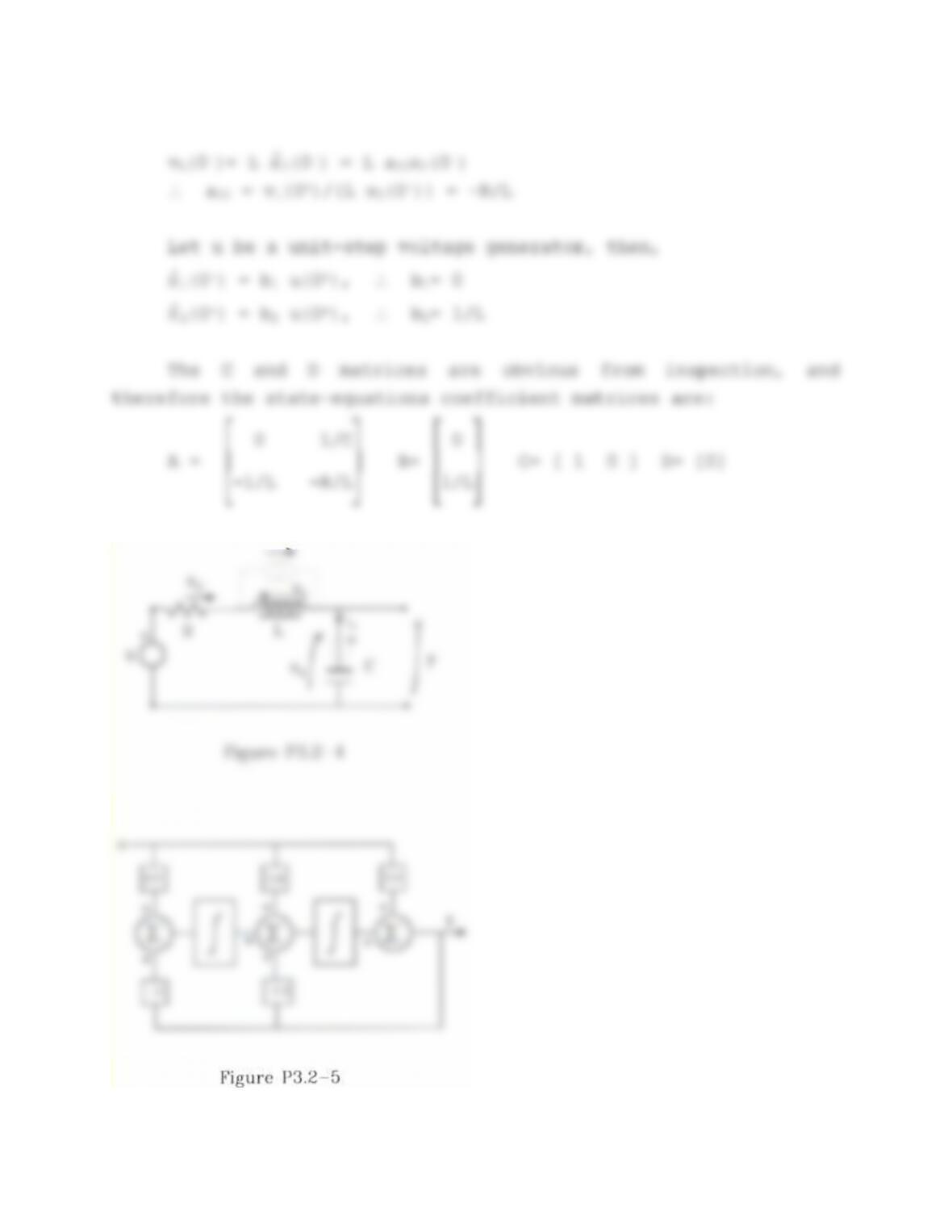
Problem 3.2-5: State equations from an ODE.
Turn the ODE into an integral equation:
.. + 3y
. + 4y = 4u
.. + 6u
. + u
Which gives the simulation diagram in Fig. P3.2-5.
Define state variables to be integrator outputs, from the right.
By inspection, the state-equation coefficient matrices are:
The A and B coefficient matrices agree with Eqn. 3.2-6.
——————-
Problem 3.2-6: Discrete time recursion formula from Simpson’s
rule.
Equation 3.2-9 is:
T
ATATA )()()1(
0
Apply the equation to two sample periods:
dkTBueekxekx
T
ATATA )()()2(
2
0
22
Approximate the integral by Simpson’s rule:
Problem 3.2-7. Find eigenvalues, eigenvectors, modal matrix, and
matrix exponential for the given matrix.
The characteristic equation is:
which gives the eigenvalues:
The adjoint matrix (transposed cofactor matrix) is:
2
1)3()43(
sss
and any nonzero column gives an eigenvector when evaluated at an
eigenvalue. The eigenvectors are:
A modal matrix is formed from the eigenvectors:
221
jj
The matrix exponential found from (3.2-12) is:
┌ ┐
——————-
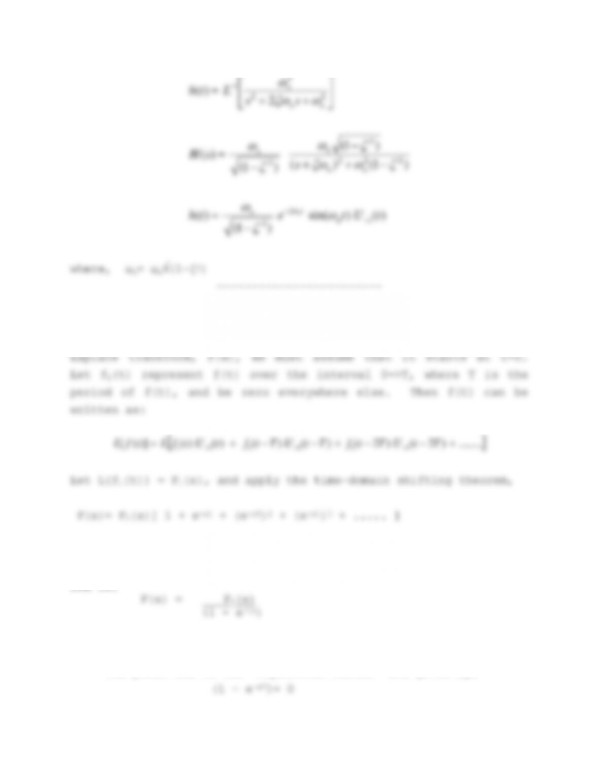
Problem 3.2-8: Matrix exponential found by Laplace transform for
Let F(s)=1/(s2+s+1) = 1/[(s+½)2 + 3/4]
then,
Therefore,
)2/3sin()3/1()2/3cos()2/3sin()3/2(
)2/3sin()3/2()2/3sin()3/1()2/3cos(
2/
ttt
ttt
In its simplest form,
)2/3sin()3/2()3/2/3sin()3/2(
2/
tt
———-———–
Problem 3.2-9: Laplace transform solution of the ODE:
y
. + y = sin(10t + α)U-1
Apply the trig. identity for sin(A+B), and the L.T. of sine and
and by comparing coefficients,
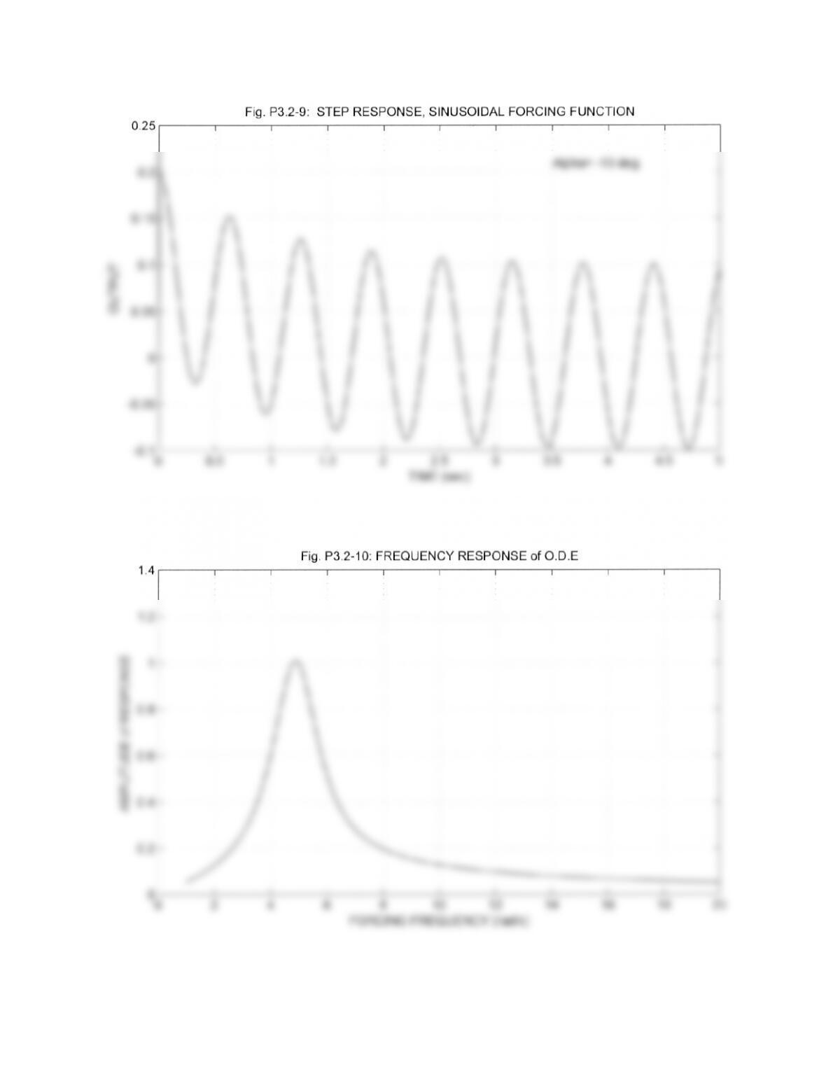
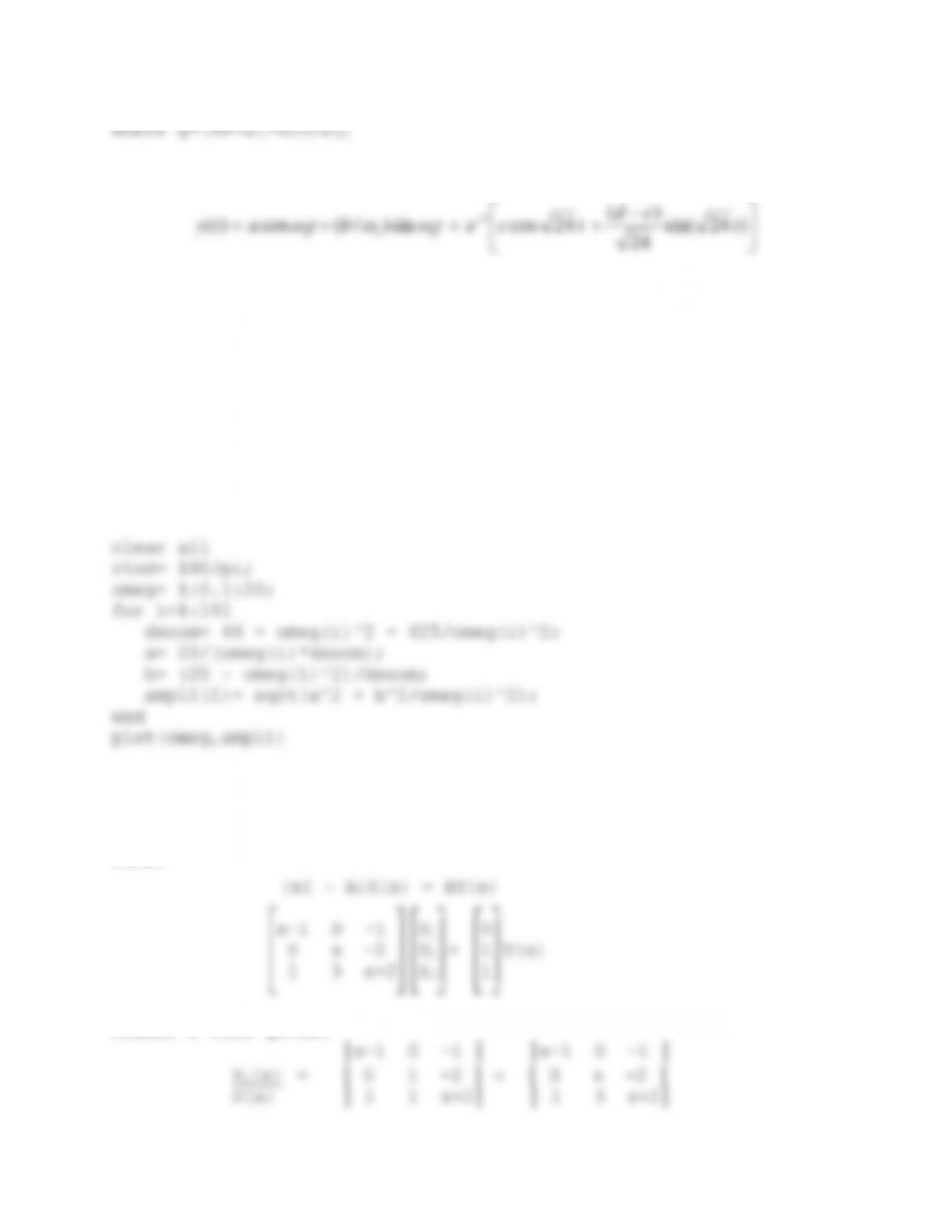
A program to plot the solution is given below, and a typical plot
is shown in Fig. P3.2-9. Trial and error shows that the largest
positive transient occurs when α -100, and α1750 gives the
% Program P329.m
clear all
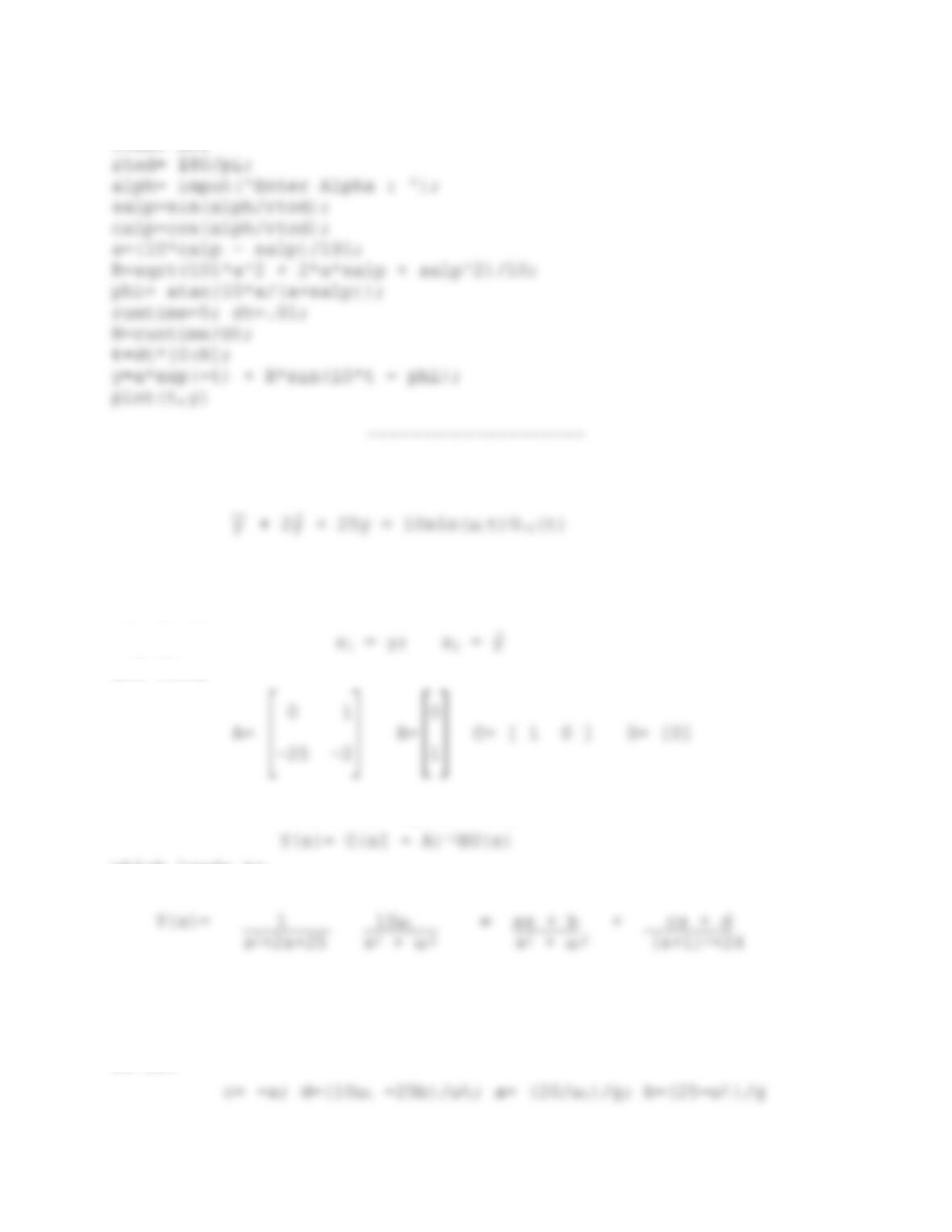
Prob. 3.2-10(a) Laplace transfm. soln. of an ODE via state eqns.
.. + 2y
. + 25y = 10sin(ω1t)U-1(t)
With no RHS derivatives it is convenient to choose phase
variables:
x
1 = y; x2 = y
.
and then,
The solution of the state equations is:
which leads to,
s2+2s+25 s2 + ω1
Note that here it is simpler to solve the ODE directly by L.T.
By comparing coefficients, the partial-fraction coeffs. are found
to be:
and the solution is:
24
)(
cd
The first two terms are the “particular integral” solution (the
response to the forcing function).
(b) Amplitude v. frequency for the particular-integral solution
A program to plot the amplitude is given below, and the plot
is shown in Fig. P3.2-10. The amplitude passes through a peak
when the forcing frequency, ω1, is near to the natural frequency
of the system at 24 rad/s. This is an example of “resonance.”
———-———-
Problem 3.3-1: Transfer function from state eqns. by Cramer’s
rule.
Cramer’s rule gives:
from which,
65
33
)(
)(
23
2
2
sss
ss
sU
sX
———-———-
Problem 3.3-2: Effect of a transfer-function zero on step
response.
For more generality, write the transfer function denominator
in standard form, the output transform is:
1
nn
s
s
sss
Comparing coefficients,
In terms of a single sinusoidal component,
A program to evaluate this expression is given below. At s=0 the
value of the transfer function is α (the d.c. gain). Therefore,
for easier comparison of the results, y(t) has been scaled by 1/α
and multiplied by sign(α). Thus, the step responses all settle at
unit amplitude, and are positive regardless of the sign of alpha.
Figure P3.3-2 shows the step response; each graph is labeled with
a value of alpha.
For α > 0, the results show that as α is reduced below about
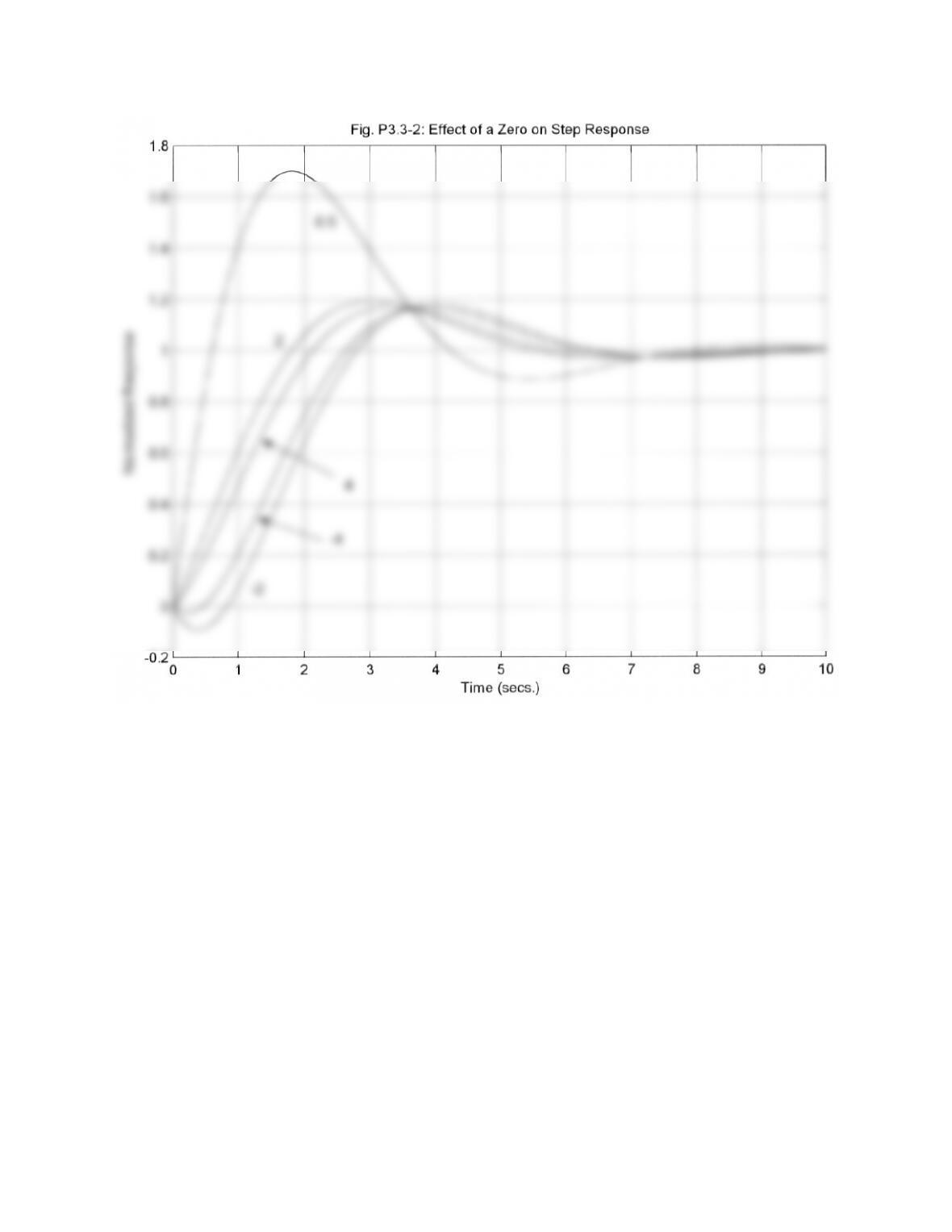
3.0 (6 times the magnitude of the real-part of the complex poles)
the overshoot (beyond 1.0) of the step response increases greatly,
and the undershoot (after the first peak) also increases. This is
accompanied by a reduction in the time to reach the peak.
For α < 0, an undershoot occurs immediately after t=0 (the
characteristic response caused by a non-minimum-phase zero). As
α is reduced below about 3.0 the undershoot increases greatly,
and this increases the time taken to reach the first peak. The
height of the first peak does not increase nearly as rapidly as
for the positive alpha case.
————————
Problem 3.3-3: Step-response of the simple-lead transfer function.
)()(
/1
11
1
)(
1
/tUety
sss
s
sY
t
———-———–
Problem 3.3-4: Unit-impulse response of the quadratic lag.
)1(
)(
2
)(
222
2
22
2
1
sH
ss
Lth
n
n
nn
n
Problem 3.3-5: Laplace transform of a “periodic” function.
(a) For the “periodic” function, f(t), to have a single-sided
The infinite geometric series converges when Re[s]>0 (the usual
condition for the existence of a single sided-Laplace), and the
sum is:
(b) Poles and zeros of F(s).
The poles due to the “repetition factor” are given by:
(1 – e
-sT)= 0
Therefore, F(s) has a pole at the origin, poles equally spaced on
the imaginary axis between -j and j, and the set of poles of
F1(s).
———-———-
Problem 3.3-6. Transfer function of the zero-order hold.
Generalize the ZOH transfer function to:
The inverse is:
This shows that the factor (1-e-Ts) will produce a rectangular
pulse of width T from a unit step, level out a unit ramp, or pick
5.
(b) Poles and Zeros of the ZOH transfer function.
The zeros of this transfer function are in the same positions
Problem 3.4-1. Comparison of ABM and Runge-Kutta integration.
The second-order ABM integration formula, programmed as a
function that is interchangeable with the 4th-order Runge-Kutta
formula given in the textbook, is:
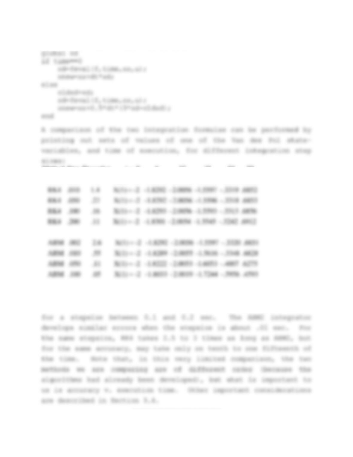
function [xnew]=ABM2(f,time,dt,xx,u)
.4593 .5956– 1.7244– 2.0019– 1.8033– -2X(1) .05 .100 ABM
.6275 .4007– 1.6053– 2.0053– 1.8222– -2X(1) .11 .050 ABM
.6828 .3348– 1.5616– 2.0055– 1.8289– -2X(1) .55 .010 ABM
.6851 .3320– 1.5597– 2.0056– 1.8292– -2X(1) 2.6 .002 ABM
.6912 .3242– 1.5545– 2.0054– 1.8301– -2X(1) .11 .200 RK4
.6856 .3313– 1.5593– 2.0056– 1.8293– -2X(1) .16 .100 RK4
.6853 .3318– 1.5596– 2.0056– 1.8292– -2X(1) .27 .050 RK4
With a stepsize of .002 the two sets of results are
essentially identical. The RK4 results develop significant errors
———-————