Therefore, if ωb/aω, the corresponding quaternion is:
——————
Problem 1.8-4: Reproduce the results of Example 1.8-3.
——————
Chapter 2
Problem 2.2-1: Calculation of airfoil Aerodynamic Center position
and Cmac.
———————
Problem 2.3-1: Effect of a gust on the aerodynamic angles.
(i) 20ft/s horizontal gust in the positive y direction:
Initially,
32.69
58.43
3.493
cossin
sin
coscos
frd
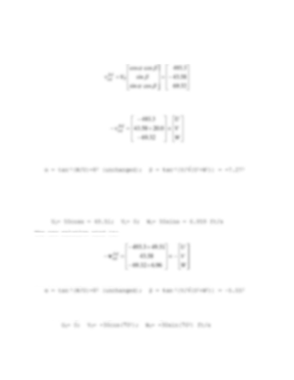
When the gust strikes, the new relative wind is:
The new aerodynamic angles are:
(ii) Horizontal gust of 50 ft/s from dead astern:
Airplane pitch attitude is θ= 80 (since γ=0). Therefore, the
body-axes components of the gust are:
The new relative wind is:
W
rel
96.632.69
and the aerodynamic angles are:
(iii) Gust of 30ft/s from below and right.
The body-axes components of the gust are:
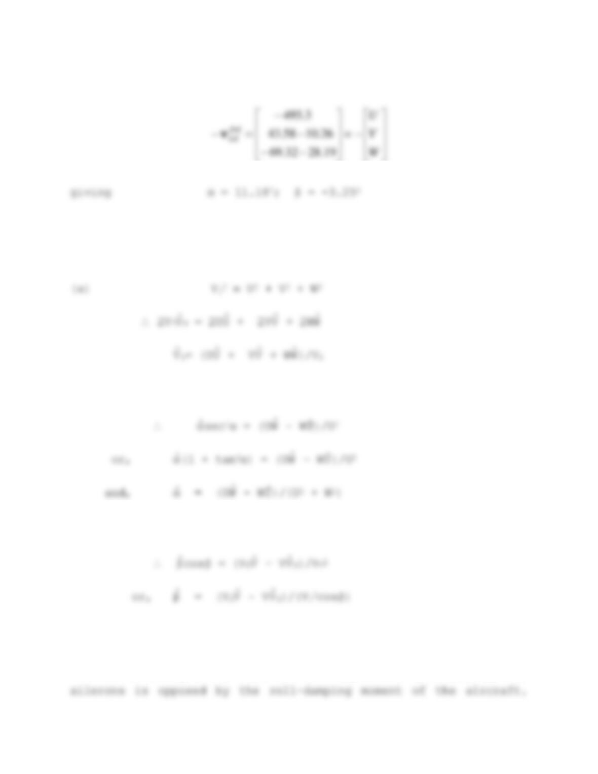
and the relative wind is:
W
V
U
frd
rel
19.2832.69
26.1058.43
3.493
v
———————–
Problem 2.3-2: Derivatives of VT, α, β
Starting from the results in Table 2.3-1, we obtain:
V
T= (UU
(b) tanα W/U
.sec2α = (UW
. – WU
.)/U2
and, α
(c) sinβ V/VT
.cosβ = (VTV
. – VV
.
———————-
Problem 2.3-3: Helix angle and Roll-Rate
In a steady-state roll the rolling moment produced by the
Thus, an approximate relationship involving the linear stability
and control derivatives is:
The helix angle, pb/(2VT), reaches its maximum with maximum aileron
with increasing airspeed, leading eventually to the condition of
“aileron reversal.”
Information on aileron control, maximum roll-rate, and helix
angle is available in the books by Perkins and Hage, and Stinton
(see page 77, Stevens & Lewis), in Hoerner (“Fluid Dynamic Lift,”
S. F. Hoerner and H. V. Borst, 2nd. Ed., 1985, p. 10-6), and the
equation (1), although a correction factor is normally applied to
this equation (see Perkins and Hage).
Note that a modern fighter will have fully-powered irreversible
control surfaces so that the maximum aileron deflection is not
limited by the pilot’s strength, but may be limited by the
automatic flight-control system.
———————-
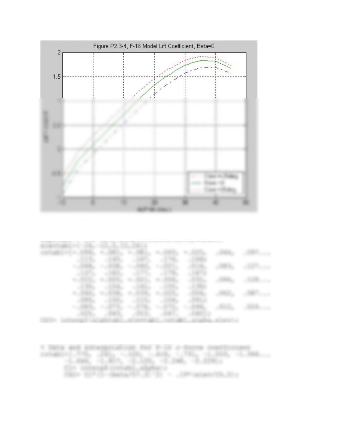
Problem 2.3-4: F-16 lift curve.
It is shown in Section 2.3 that the lift coefficient is given
by:
The tabular values of the coefficients CX and CZ given in
Appendix-A were coded as function subprograms as shown below, and
another m-file was written to combine and plot them. In the
figure, the maximum of the lift curve occurs between 350 and 400
alpha, depending on the elevator setting. Note that the inter-
polation routines do not allow extrapolation, and the data only
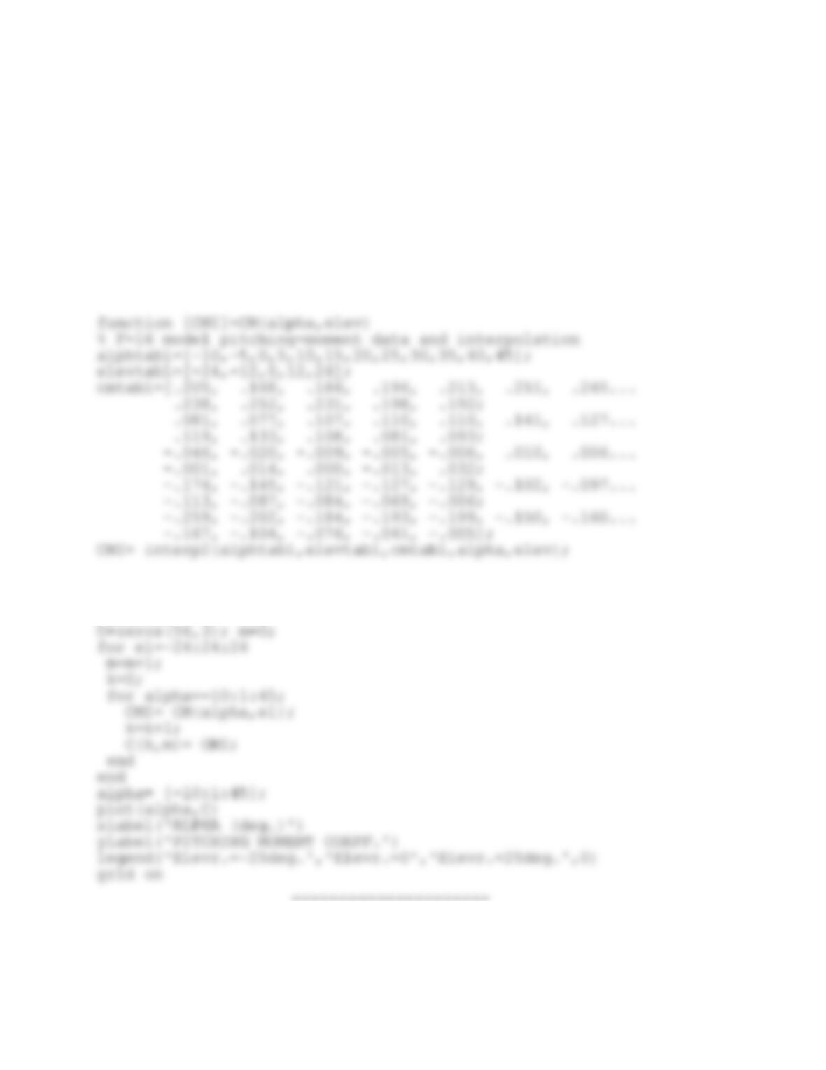
function [CXI]=CX(alpha,elev)
% Data and interpolation for F-16 Axial force coefficient.
alphtabl=[-10,-5,0,5,10,15,20,25,30,35,40,45];
function [CZI]=CZ(alpha,beta,elev)
% Program to plot F-16 lift coefficient
clear all
———————–
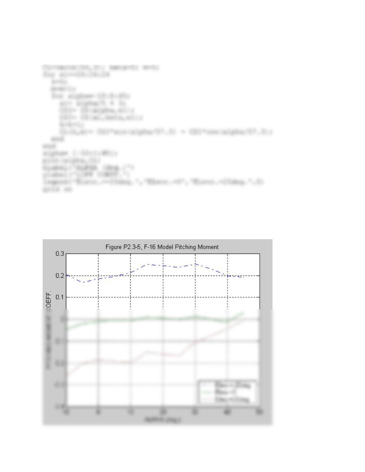
2.3-5 F-16 pitching moment curve:
The pitching moment coefficient is the same in either the body-
fixed or the stability axes, and is the coefficient CM(alpha,el)
given in Appendix A. Programs to interpolate and plot the
pitching moment data are given below. The plot above shows that
the aircraft does not have positive pitch stiffness over much of
the normal range of angle-of-attack, and also shows the
deterioration in elevator effectiveness (loss of nose-down
pitching moment control) at high alpha.
% Program to plot F-16 pitching-moment data
clear all
———————
2.3-6 F-16 engine thrust model:
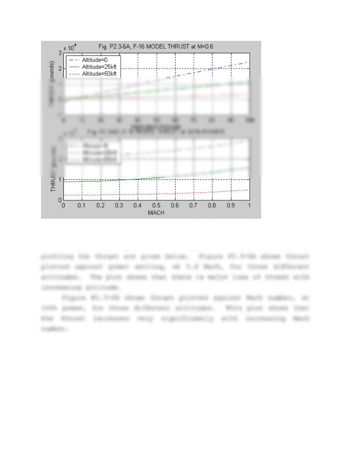
The engine thrust model is the FORTRAN function THRUST(POW,AL-
T,MACH) given in Appendix A. Programs for interpolating and
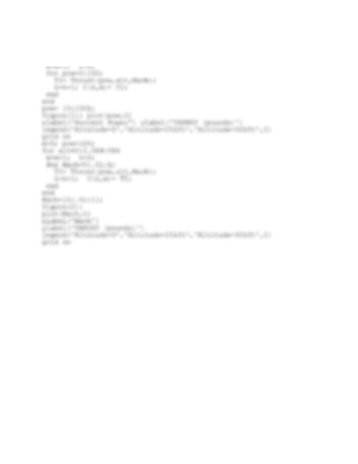
%Program to plot F-16 engine model thrust
clear all; C=zeros(101,3); Mach=0.6; m=0;
for alt=0:2.5E4:5E4
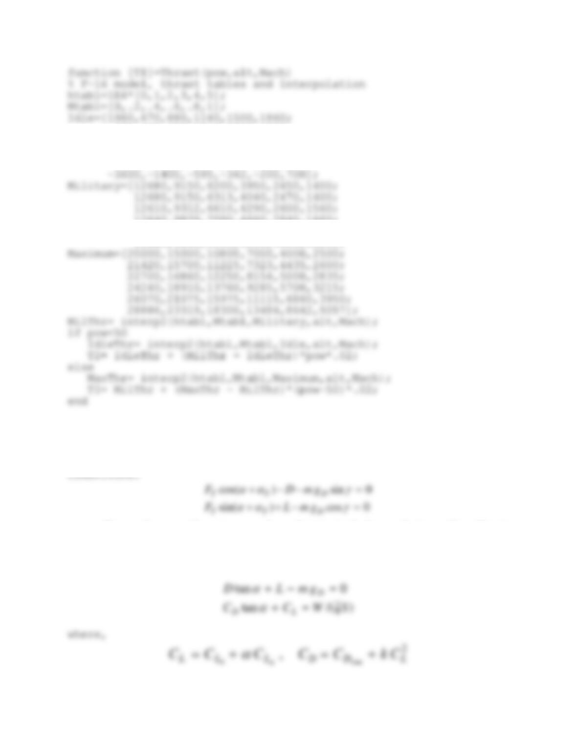
635,425,690,1010,1330,1700;
60,25,345,755,1130,1525;
-1020,-710,-300,350,910,1360;
-2700,-1900,-1300,-247,600,1100;
12640,9839,7090,4660,2840,1660;
12390,10176,7750,5320,3250,1930;
11680,9848,8050,6100,3800,2310];
Problem 2.4-1: Solution of nonlinear steady-state flight eqns.
Equations 2.5-32 give the longitudinal equilibrium
DTT
gmLF
The unknown thrust can be eliminated by solving the first
equation for FT and substituting in the second equation. Then,
since 0 T
, we obtain,
min0 ,LDDLLL CkCCCCC
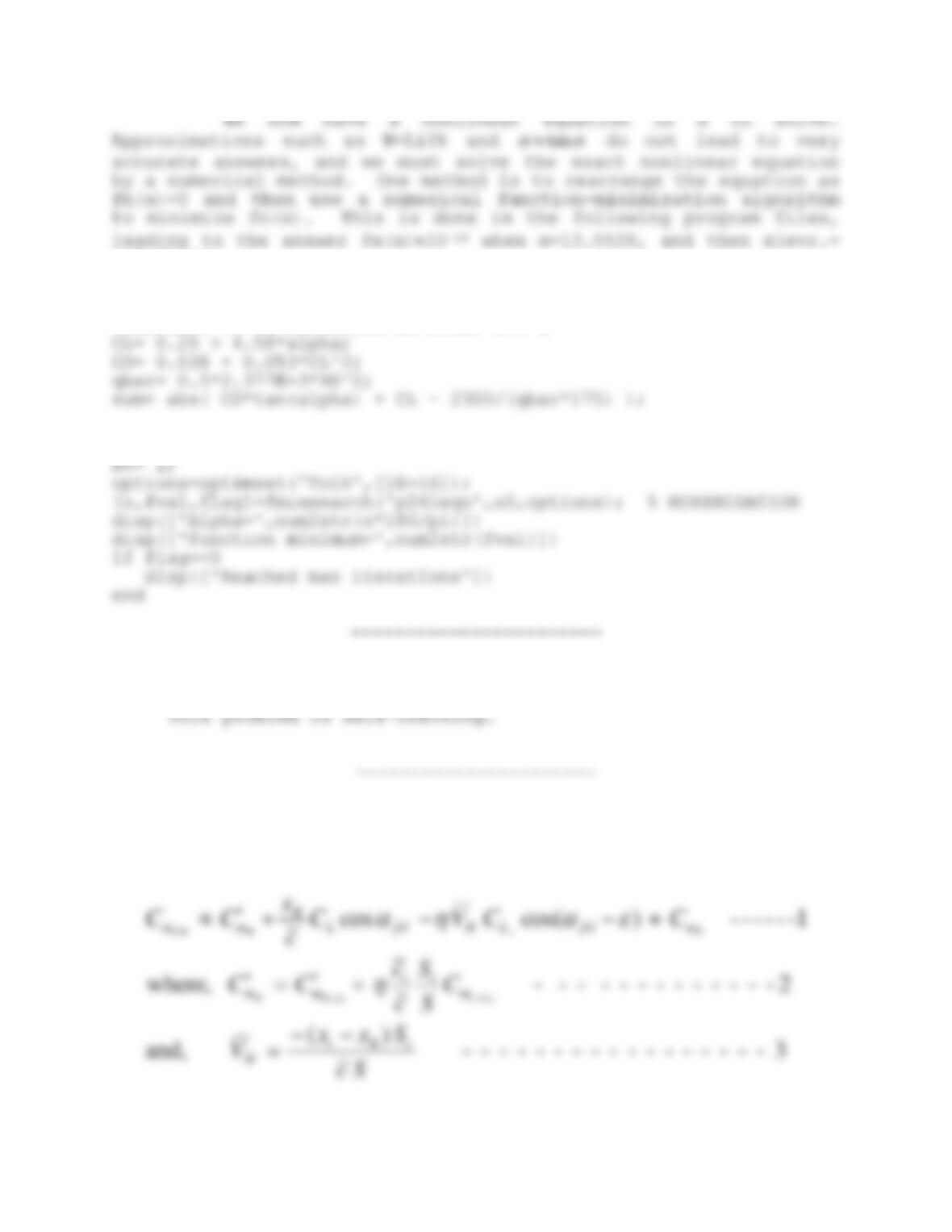
-10.34 deg.
function [sum]= P241eqn(alpha)
%Function to be minimized in Prob. 2.4-1
%Program to solve Prob. 2.4-1
Problem 2.4-2: Derivation of Eqn. 2.4-13.
Problem 2.4-3: Calculation of airspeed in steady-state flight.
Equation 2.4-15 is applicable to this problem:
2– – – – – – – – – – – – – ,where
-1––––– )cos(cos
,4/,
C
S
c
CC
CCVC
c
x
CC
m
tt
mm
mfrlLHfrlL
R
mm
tcwbRR
PtRCM
In the problem statement, take the references to the “wing” as
meaning wing-body combination. Also, make small angle approxima-
tions so that the cosine terms in (1) are unity. Neglect the
propulsion term in (1), and the tail component in (2).
Now, take the aerodynamic data reference point, R, as the ac
of the wing and body, so that (1) becomes:
t
twbacCM
L
t
wb
LL
LHL
ac
mm
C
S
S
CC
CVC
c
x
CC
where,
4– – – – – – – – – –
,
Substituting the equilibrium values in (4) gives:
(b) Airspeed for trimmed flight:
For equilibrium at small alpha weight=lift, therefore,
———————-
Problem 2.5-1: Block diagram of the flat-Earth equations.
Figure P2.5-1 shows the block diagram of the flat-Earth
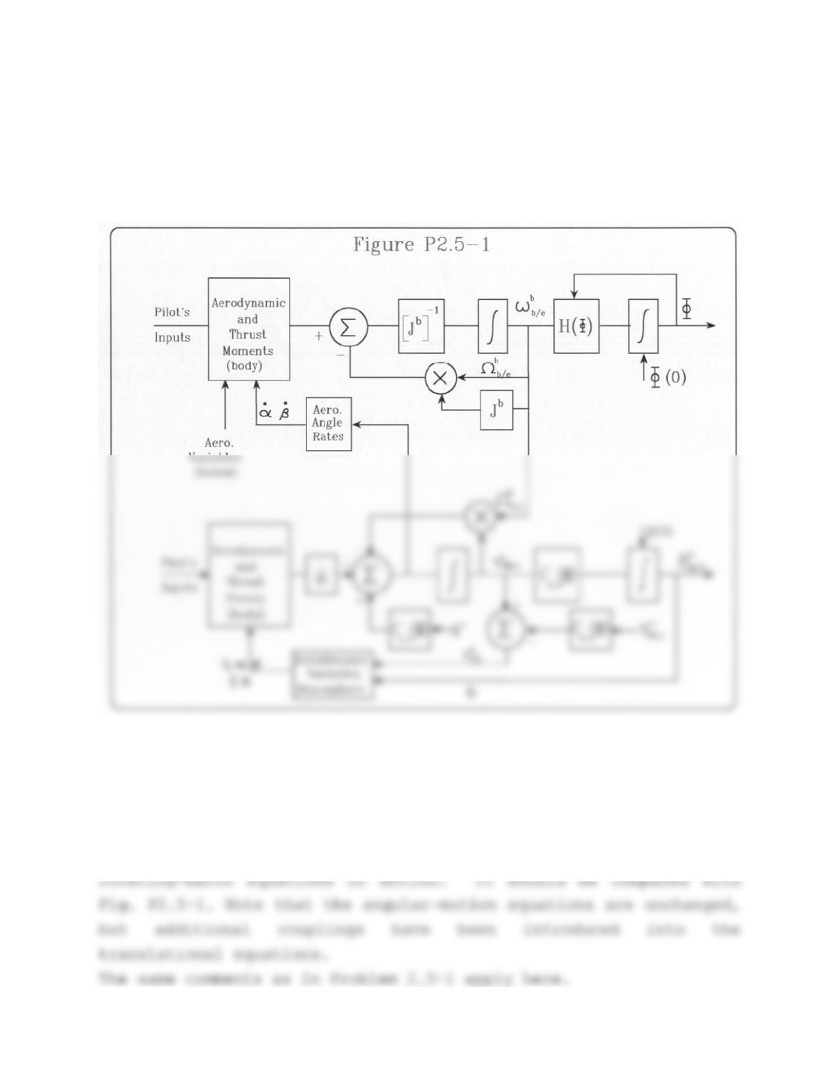
coupling occurs between the angular and translational motions. It
is also helpful in considering different choices of state-
variables, in constructing a simulation, and in organizing the
equations to minimize the number of mathematical operations.
————————
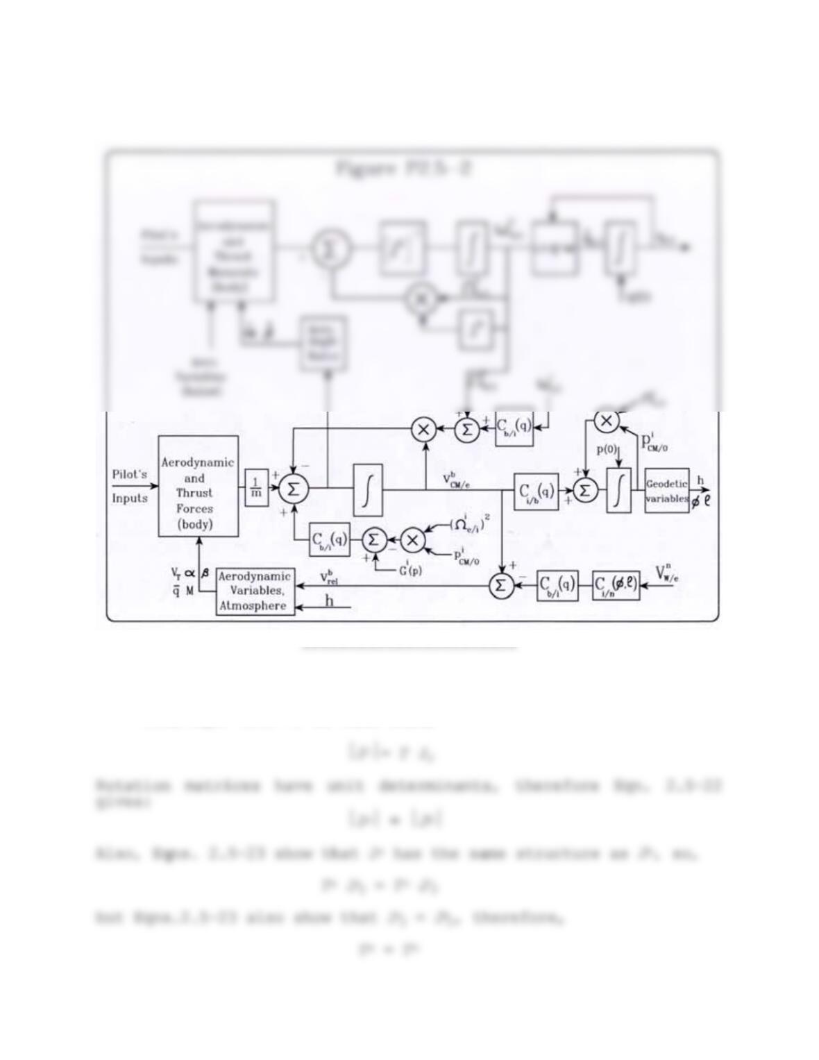
Problem 2.5-2: Block diagram of the oblate, rotating-Earth eqns.
Figure P2.5-2 shows the block diagram of the oblate,
Problem 2.5-3: Calculation of Γ in the moment equations.
From Eqn. (1.5-7) we find that,
Problem 2.5-4: Expansion of the flat-Earth vector equations.
Problem 2.6-1: Linearization of the force equations.
Problem 2.6-2: Linearization of the kinematic equations.
Problem 2.6-3: Linearization of the moment equations.
Problem 2.6-4: Numerical calculation of a derivative.
The derivative of a continuous function can be estimated by
using finite differences. For the continuous function g(v), the
simplest approximation to the derivative at v=a is given by the
first difference (see Chap. 3, Sect. 7) :
where h is made as small as possible without incurring round-off
errors due to finite-precision computer arithmetic.
interpolated Cm table used in Problem 2.3-5 is given below.
% Program to estimate a derivative
a= input(‘Enter alpha : ‘),
da= 1.0; tol=1E-6;
last=0; el=0;
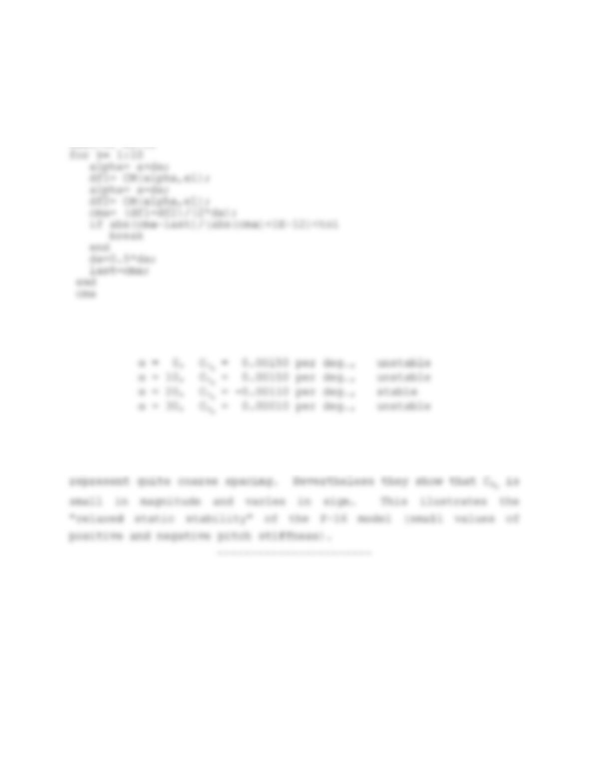
The results obtained with this program were:
These results are not necessarily very good estimates of the true
Cmα because the 50 alpha-increments of the aerodynamic data