Problem 1.6-5: Conditions for geostationary orbit.
An orbit with constant angular rate, matching that of the
Earth (i.e. geostationary), must be circular. The forces can only
remain balanced if the center of the orbit is at the Earth’s cm
(i.e. a great circle orbit), and the latitude can only remain
constant if the orbit is over the equator.
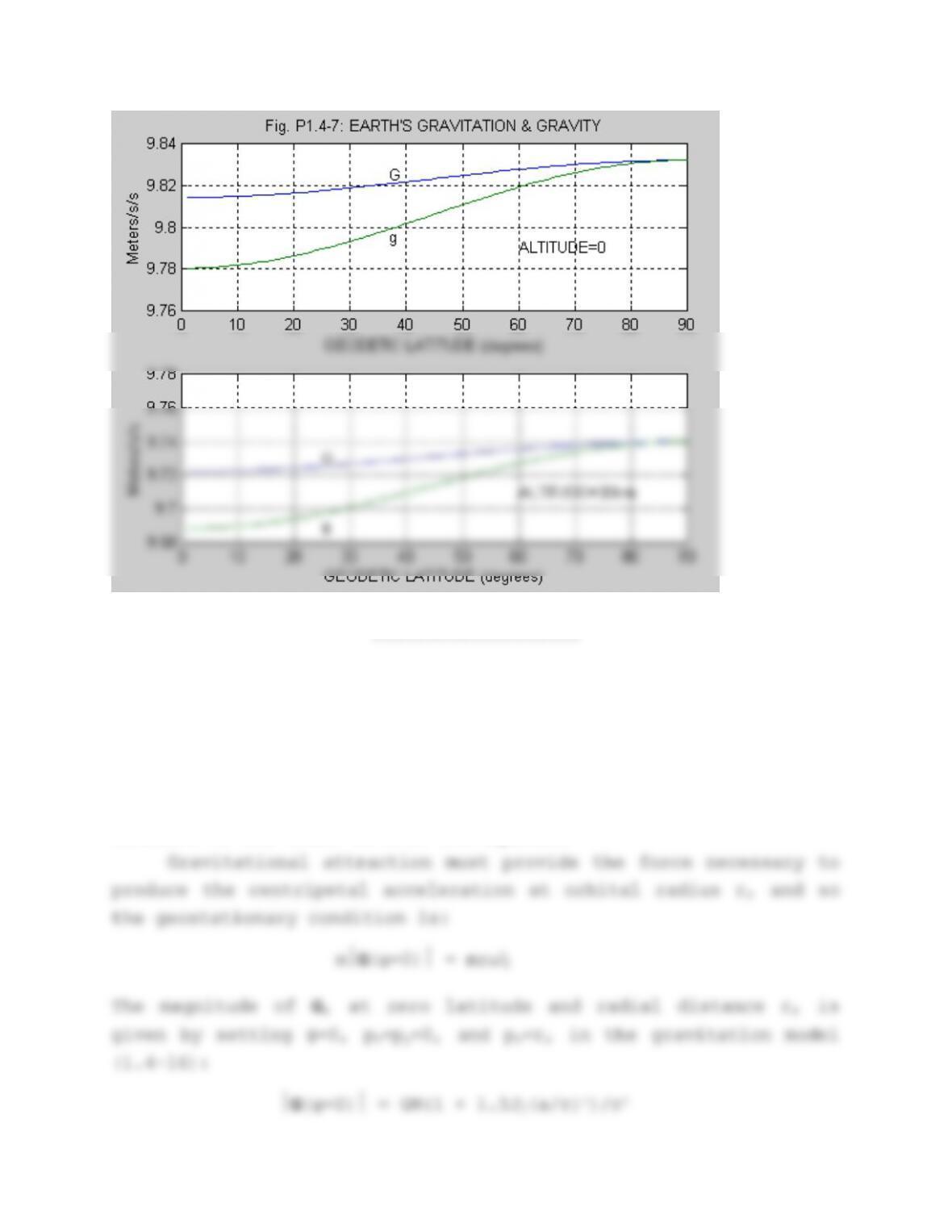
Substituting this into the geostationary condition gives:
The J2 term has an almost negligible effect on the answer. An
“official” figure for the height is 22,236.46 miles (IEEE
Spectrum, Sept. 1984, p.16), and the orbital speed is 3.1 km/s.
——————-
SECTION 1.7: RIGID BODY DYNAMICS
Problem 1.7-1: Aircraft mounted on a torsional pendulum.
(a) Distance of cm from nose:
Assume that the centers of mass of the individual pieces
(fuselage and wings) are evident from symmetry. Let the length of
the fuselage be l and, for the whole aircraft, let the distance of
the cm from the nose be x units. Now, taking moments of the wings
and fuselage around the aircraft z-axis (passing through the
aircraft cm, and positive down), we have,
(b) Aircraft moment of inertia around the z axis
Approximate the fuselage and wings by rectangular paral-
lelepipeds with uniform mass distribution, and use the parallel-
axis theorem to find their moments of inertia around the aircraft
z-axis:
2
9
12
3
3
9
12
3
which gives,
(c) Period of the torsional oscillation:
——————–
Problem 1.7-2: Simulation of a spinning brick.
Let the axes be aligned parallel to the edges of the brick,
so that they are principal axes. If the mass of the brick is M,
the moments of inertia are:
R
where P, Q, and R are the body-axes components of the angular
velocity of the body, with respect to an “inertial” reference
frame.
The Euler kinematical equations provide the angular rates φ
.,θ
.
. When these rates are integrated the Euler angles may fall
convenience of interpretation and to avoid eventual numerical
problems, the angle state-variables must be modified, before or
after the numerical integration; for example,
where “rem” is the computer remainder function. This angle
modification does not introduce a discontinuity into the
trigonometric functions, and so will not normally cause difficulty
for i=0:N
P= X(4); Q= X(5); R= X(6);
if rem(i,NP)==0 % Get output
k= k+1;
y(k,1)= P; y(k,2)= Q; y(k,3)= R;
z(k,1)= rtod*X(1); z(k,2)= rtod*X(2);
end
toc
t= NP*dt*[0:k-1];
figure (1)
plot(t,y)
Simulation Results
Case(a): Initial conditions P=0.1, Q=0, and R=0.001 rads/sec
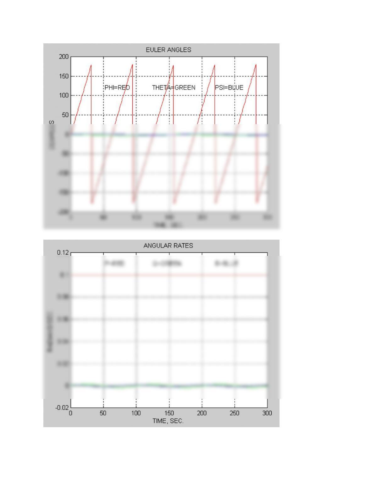
P remains constant, and so φ varies linearly from –π to π and
Case(b)(not plotted):Initial conditions P=0.001,Q=0,R=0.1 rads/sec
like case (a) but now ψ cycles linearly between ±π.
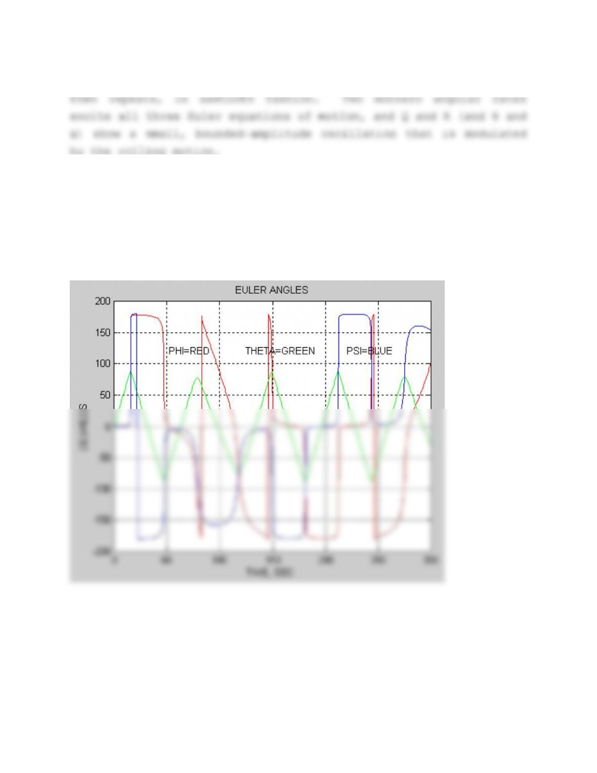
Case(c) : Initial conditions P=0.0, Q=0.1, and R=0.001 rads/sec
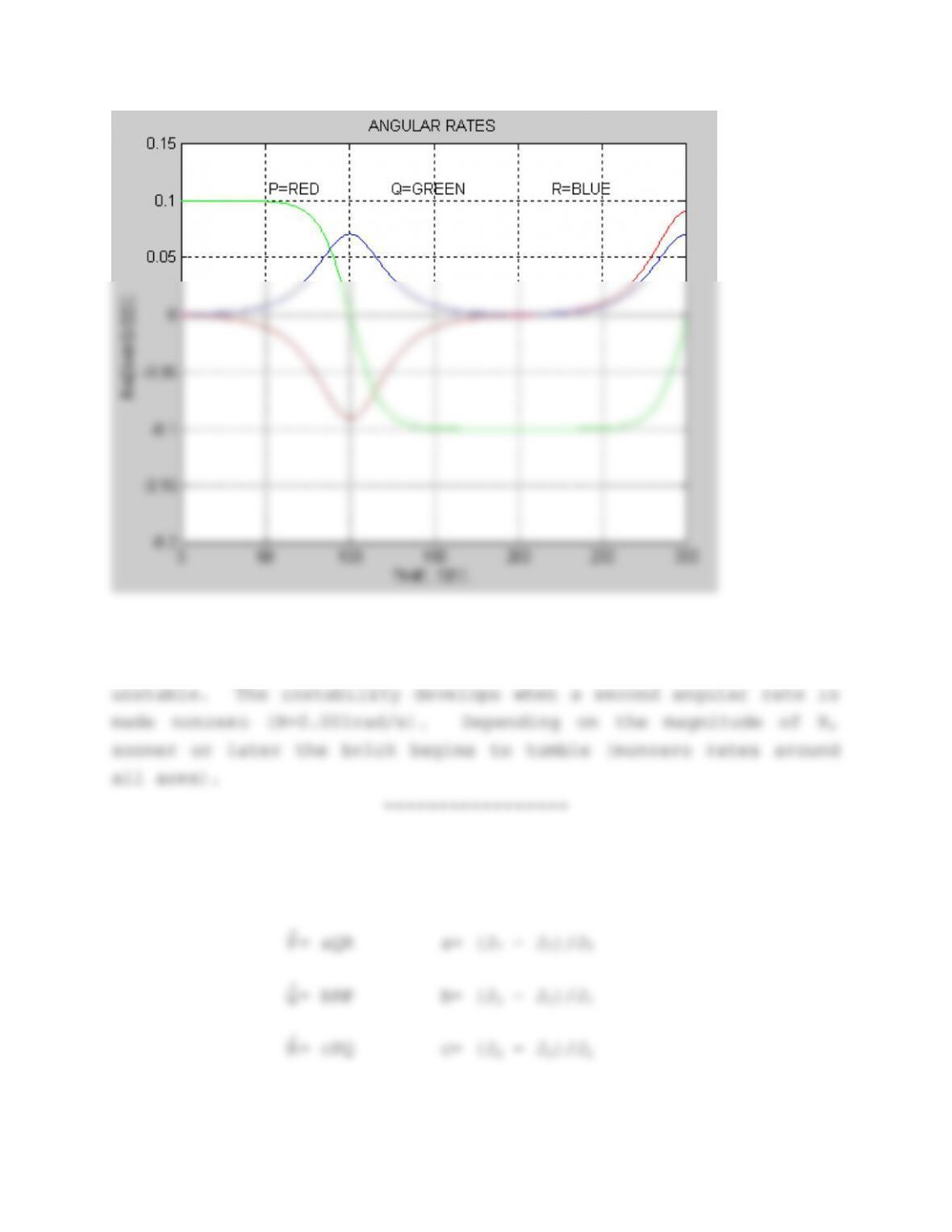
The initial rate, Q, is around the axis with the intermediate
value of the moments of inertia, and so the motion will be
Problem 1.7-3: Linearization of Euler’s equations of motion.
Rewrite Equations 1.5-6, with zero applied torques, as:
.= aQR a= (JY – JZ)/JX
R
Linear state equations can be obtained by using a Taylor-series
expansion of the nonlinear equations according to:
r
r
R
R
Q
R
P
R
where derivatives beyond the first have been neglected and lower
case symbols represent deviations of the angular rates from the
values Pe, Qe, and Re. Substituting for the partial derivatives
using Euler’s equations gives:
r
q
p
cPcQ
bPbR
aQaR
r
q
p
0
0
0
The stability of these equations is determined by the eigenvalues
of the coefficient matrix, which are given by the roots of
(which is symmetric in P, Q, and R). Consider the case when only
P is non-zero (spin about the x-axis), the roots are given by:
2
1
2
1))((
)(;0
yxxz
JJJJ
PbcP
If JX is either the largest or the smallest inertia then the
quantity in the brackets is negative, and there are two conjugate
roots on the imaginary axis. These correspond to constant rate
rotation around the x-axis. If JX lies in between the other
inertias the quantity in the brackets is positive, the roots are
then real, with equal magnitude and opposite sign. This indicates
that the motion consists of a mode that is dying out and a mode
that is growing, i.e. the motion around the x-axis is unstable.
—————–
Problem 1.7-4: Inertia coupling effect of engine angular
momentum.
R
——————–
Problem 1.7-5: Position errors of Tangent-Plane Coordinates.
Assume flight at constant altitude, h, in the Tangent Plane.
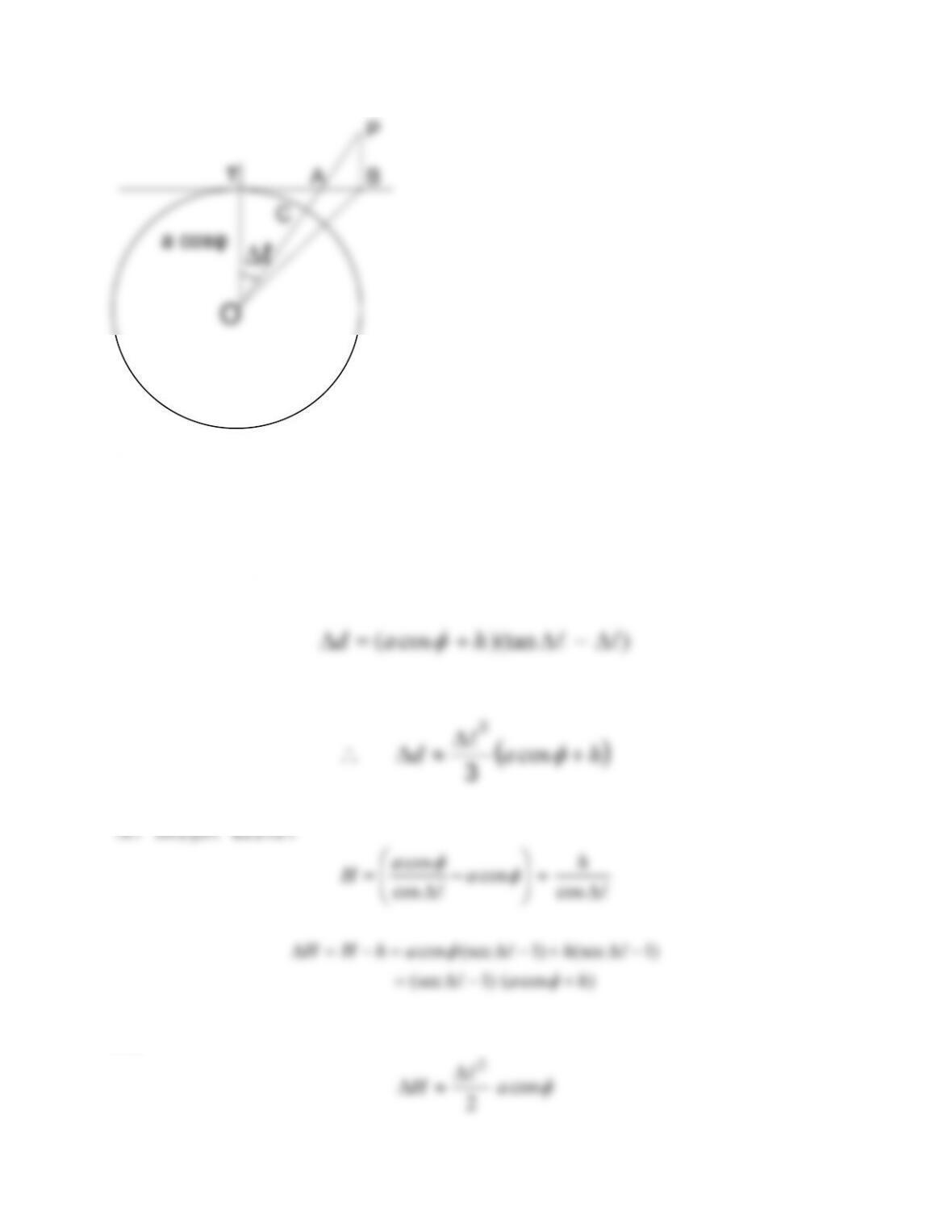
Define distance Error: lengthArcTCTBd
Tangent-plane height, h≡PB; True Height, H≡ CA + AP
Define height error as H-h
(a) Distance Error:
3
ha
So,
cos
2
2
aH
O
P
T
A
C
B
∆ℓ
a cosφ
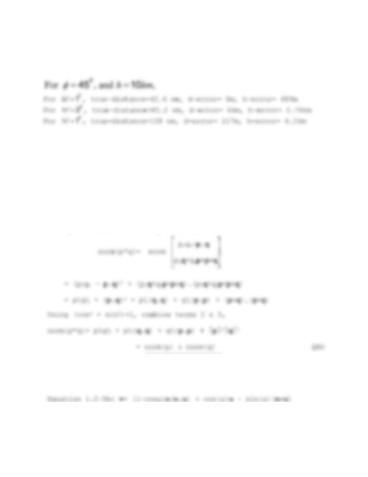
(c) Relative Significance of the errors
Conclusion: Height errors are much more significant than position
errors, but if height errors are not important then T-P
coordinates could be used for simulations up to about 100nm.
——————–
SECTION 1.8: ADVANCED TOPICS
Problem 1.8-1: Norm of a quaternion product.
By definition of multiplication,
——————
Problem 1.8-2: Operation count for rotation of a vector.
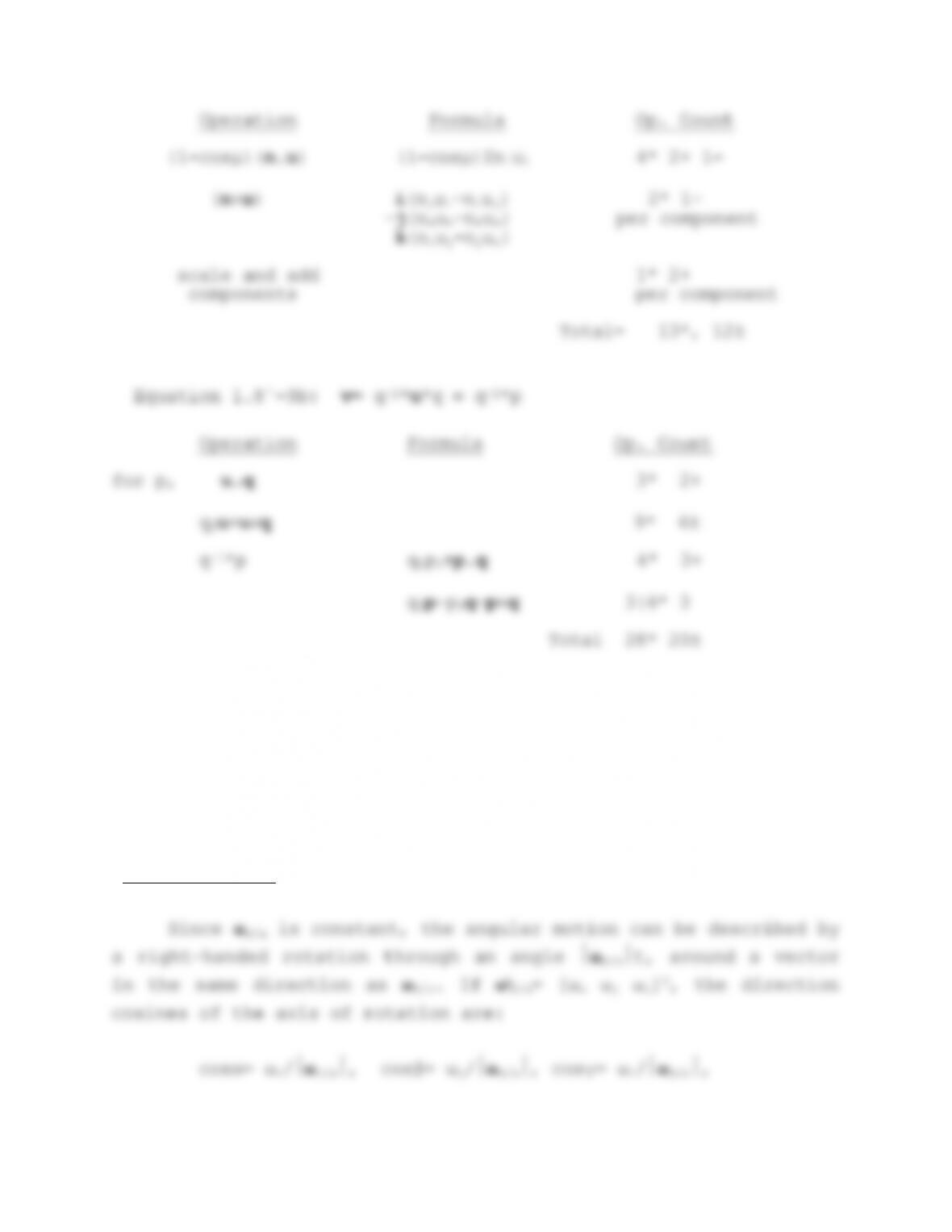
The quaternions have advantages as described in the text, and
formulae that are compact, but may require larger numbers of basic
mathematical operations than the alternatives.
—————–
1.8-3: Quaternion for constant anqular velocity rotation
(For simplicity, stipulate that the systems are aligned at t=0)