*PROBLEM 6-7B (Continued)
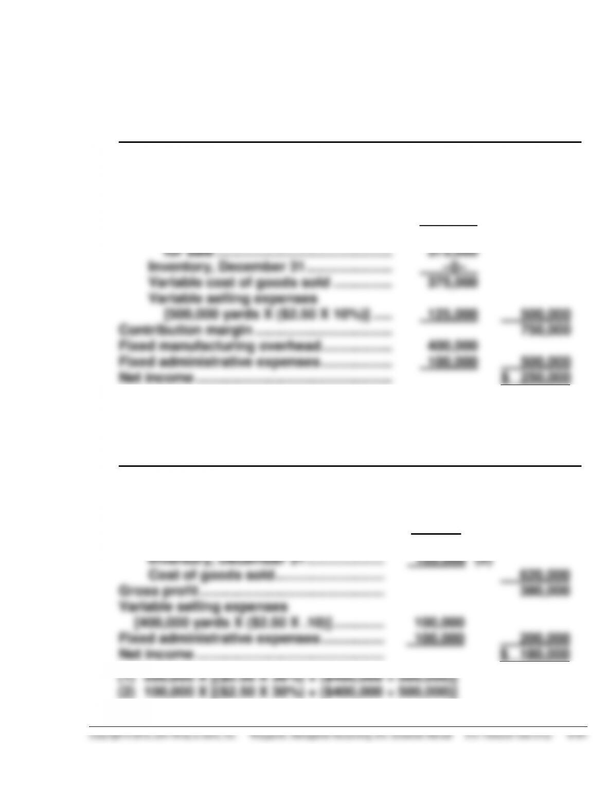
FAB COMPANY
Income Statement
For the Year Ended December 31, 2014
Variable Costing
Sales (500,000 yards X $2.50) ………………..
Variable cost of goods sold
Inventory, January 1 ………………………
Variable cost of goods manufactured
[400,000 yards X $2.50 X 30%] ……..
Variable cost of goods available
for sale ………………………………………
Inventory, December 31 ………………….
Variable cost of goods sold ……………
Variable selling expenses
[500,000 yards X ($2.50 X 10%)] …..
Contribution margin ……………………………..
Fixed manufacturing overhead ………………
Fixed administrative expenses ………………
Net income …………………………………………..
$ 75,000
300,000
375,000
–0–
375,000
125,000
400,000
100,000
$1,250,000
500,000
750,000
500,000
$ 250,000
(b) FAB COMPANY
Income Statement
For the Year Ended December 31, 2013
Absorption Costing
Sales (400,000 yards X $2.50) ………………
Cost of goods sold
Inventory, January 1 …………………….
Cost of goods manufactured…………
Cost of goods available for sale
Inventory, December 31 ………………..
Cost of goods sold ……………………….
Gross profit ………………………………………..
$ –0–
775,000
775,000
155,000
(1)
(2)
$1,000,000
620,000
380,000
*PROBLEM 6-7B (Continued)
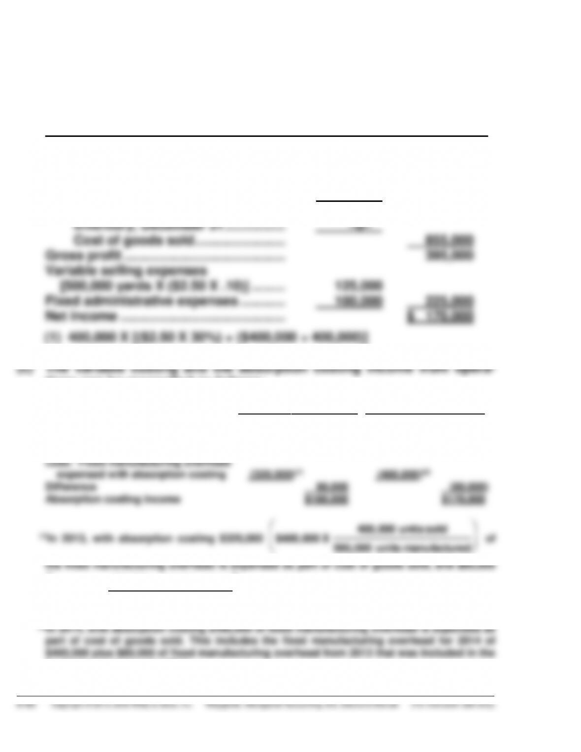
FAB COMPANY
Income Statement
For the Year Ended December 31, 2014
Absorption Costing
Sales (500,000 yards X $2.50) …………..
Cost of goods sold
Inventory, January 1 …………………
Cost of goods manufactured ……..
Cost of goods available for sale …
Inventory, December 31 …………….
Cost of goods sold ……………………
Gross profit …………………………………….
Variable selling expenses
[500,000 yards X ($2.50 X .10)] ………
Fixed administrative expenses …………
Net income ……………………………………..
$ 155,000
700,000
855,000
–0–
125,000
100,000
(1)
$1,250,000
855,000
395,000
225,000
$ 170,000
(1) 400,000 X [($2.50 X 30%) + ($400,000 ÷ 400,000)]
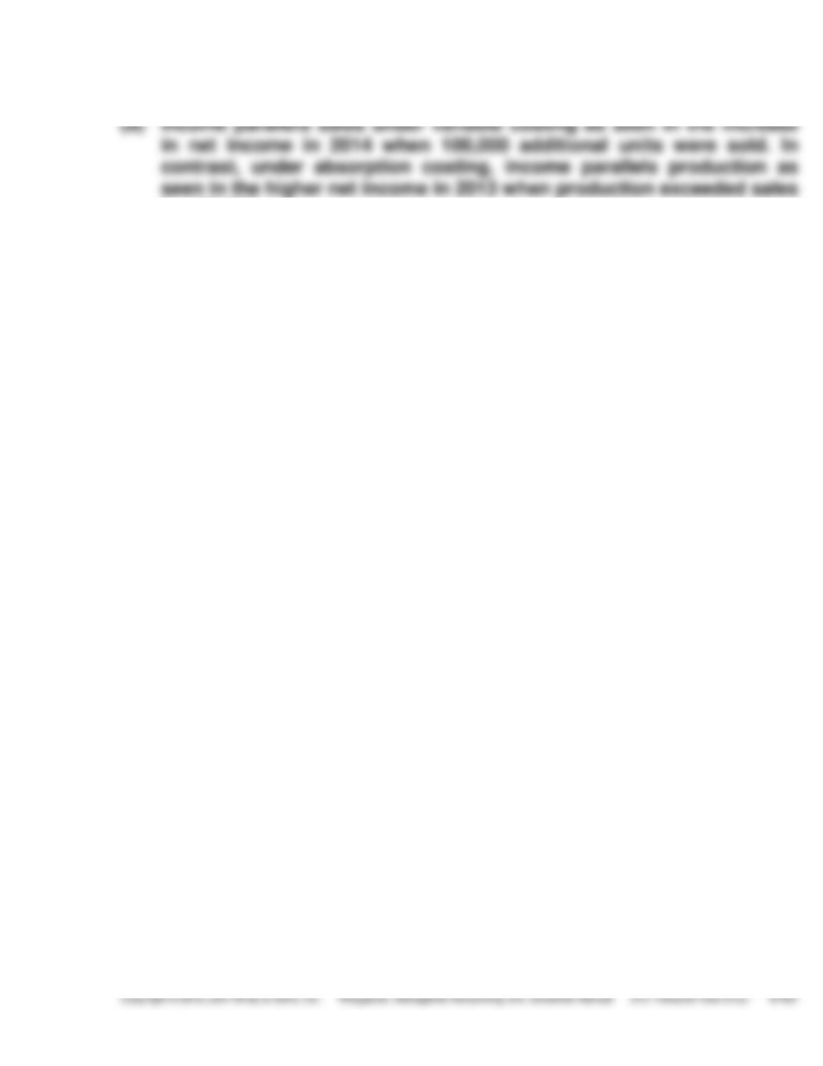
tions can be reconciled as follows:
2013
2014
Variable costing net income
Fixed manufacturing overhead
expensed with variable costing
Less: Fixed manufacturing overhead
expensed with absorption costing
Difference
Absorption costing income
$400,000
(320,000
)(1)
$100,000
80,000
$180,000
$400,000
(480,000
)(2)
$250,000
(80,000
$170,000
)
(1)In 2013, with absorption costing $320,000
$400,000 X 400,000 units sold
500,000 units manufactured
of
$400,000 X 100,000 units in inventory
500,000 units produced
is included in the ending inventory.
beginning inventory for 2014.
*PROBLEM 6-7B (Continued)
by 100,000.
*PROBLEM 6-8B
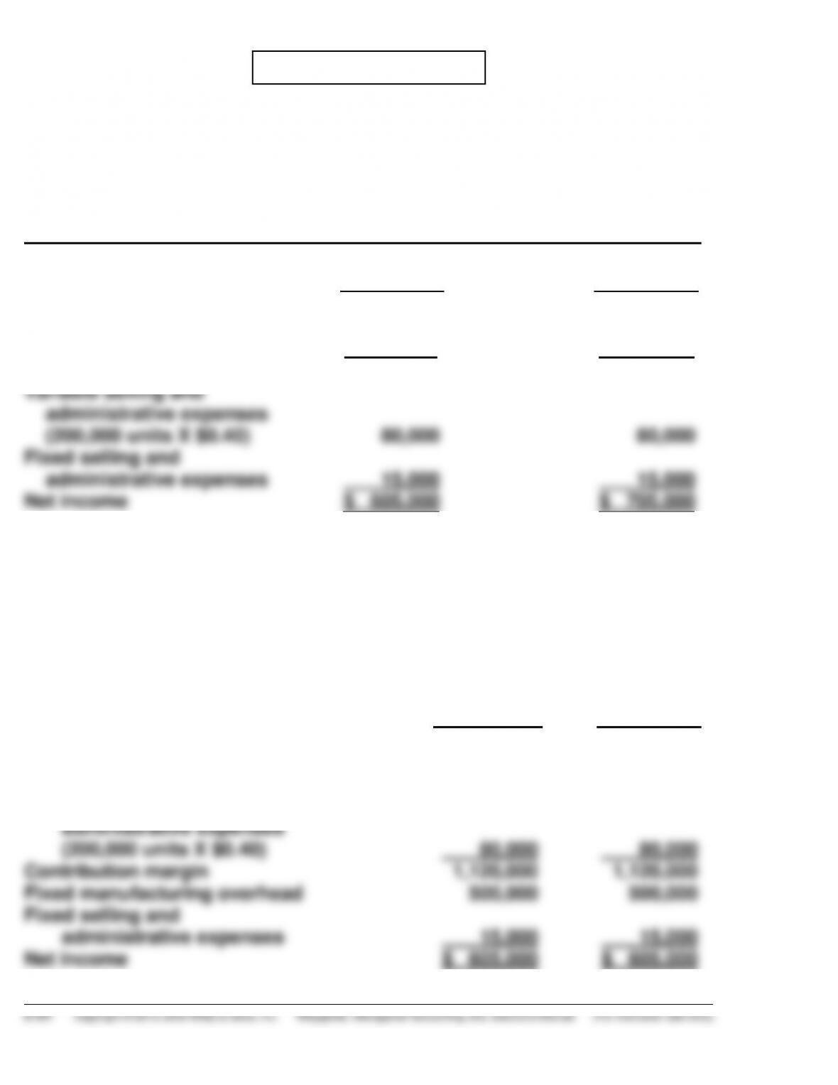
(a)
ELECTRICOIL DIVISION
Income Statement
For the Year Ended December 31, 2014
Absorption Costing
200,000 250,000
Produced Produced
Sales (200,000 units X $9) $1,800,000 $1,800,000
Cost of goods sold
(200,000 units X $5.50) 1,100,000 (200,000 X $5.00) 1,000,000
Gross profit 700,000 800,000
(b)
ELECTRICOIL DIVISION
Income Statement
For the Year Ended December 31, 2014
Variable Costing
_______________________________________________________________
200,000 250,000
Produced Produced
Sales (200,000 units X $9) $1,800,000 $1,800,000
Variable cost of goods sold
(200,000 units X $3) 600,000 600,000
Variable selling and
*PROBLEM 6-8B (Continued)
(c) If the company produces 250,000 units, but only sells 200,000 units,
then 50,000 units will remain in ending inventory. Under absorption
costing these 50,000 units will each include $2.00 of fixed manufacturing
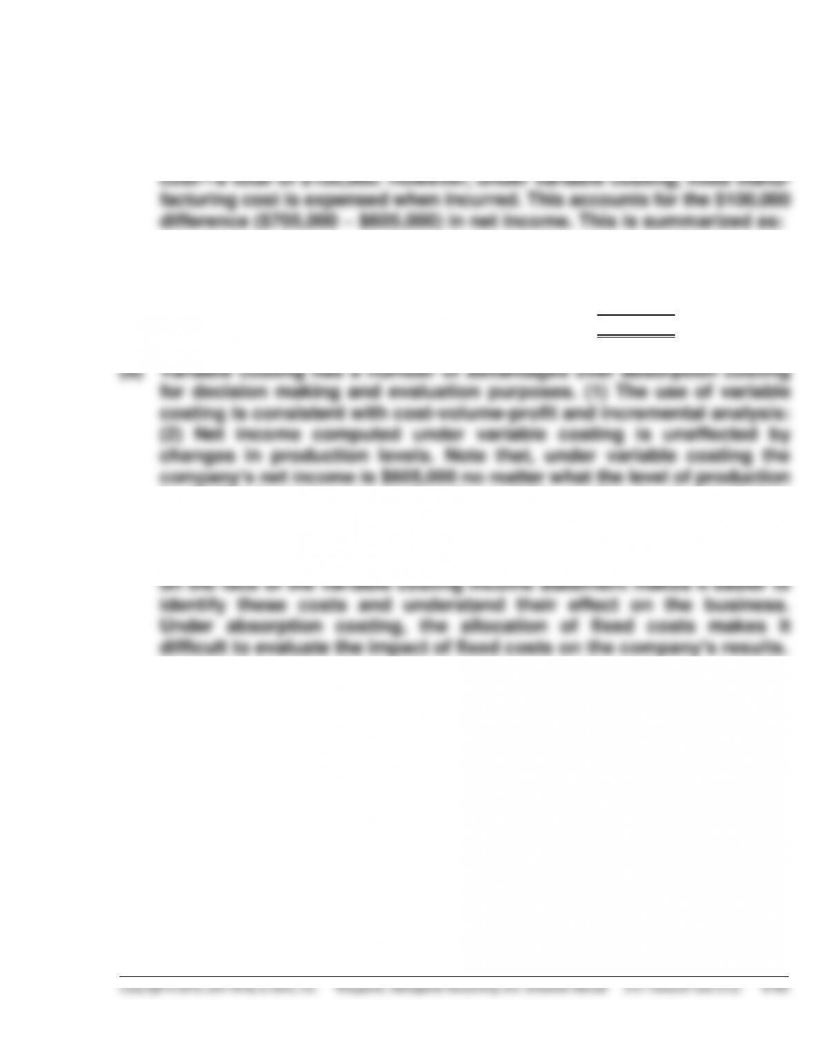
Net income under absorption costing $705,000
Less: Fixed manufacturing cost included
in ending inventory 100,000
Net income under variable costing $605,000
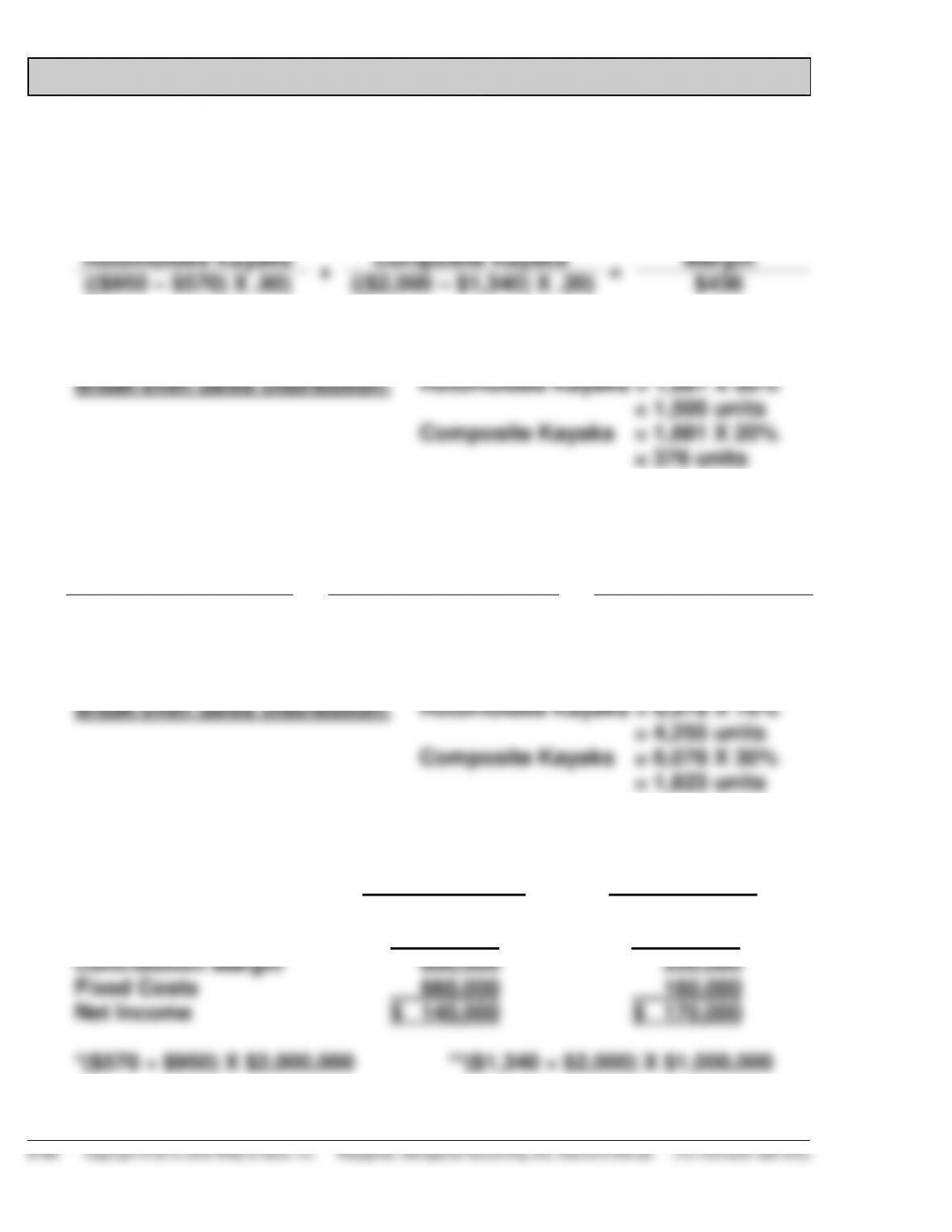
is. (3) Net income computed under variable costing is closely tied to
changes in sales levels (not production levels), and therefore provides
a more realistic assessment of the company’s success or failure during
a period. (4) The presentation of fixed and variable cost components
BYP 6-1 DECISION-MAKING AT CURRENT DESIGNS
(a)
Rotomolded Kayaks
+
Composite Kayaks
=
Weighted
Average Unit
Contribution
Margin
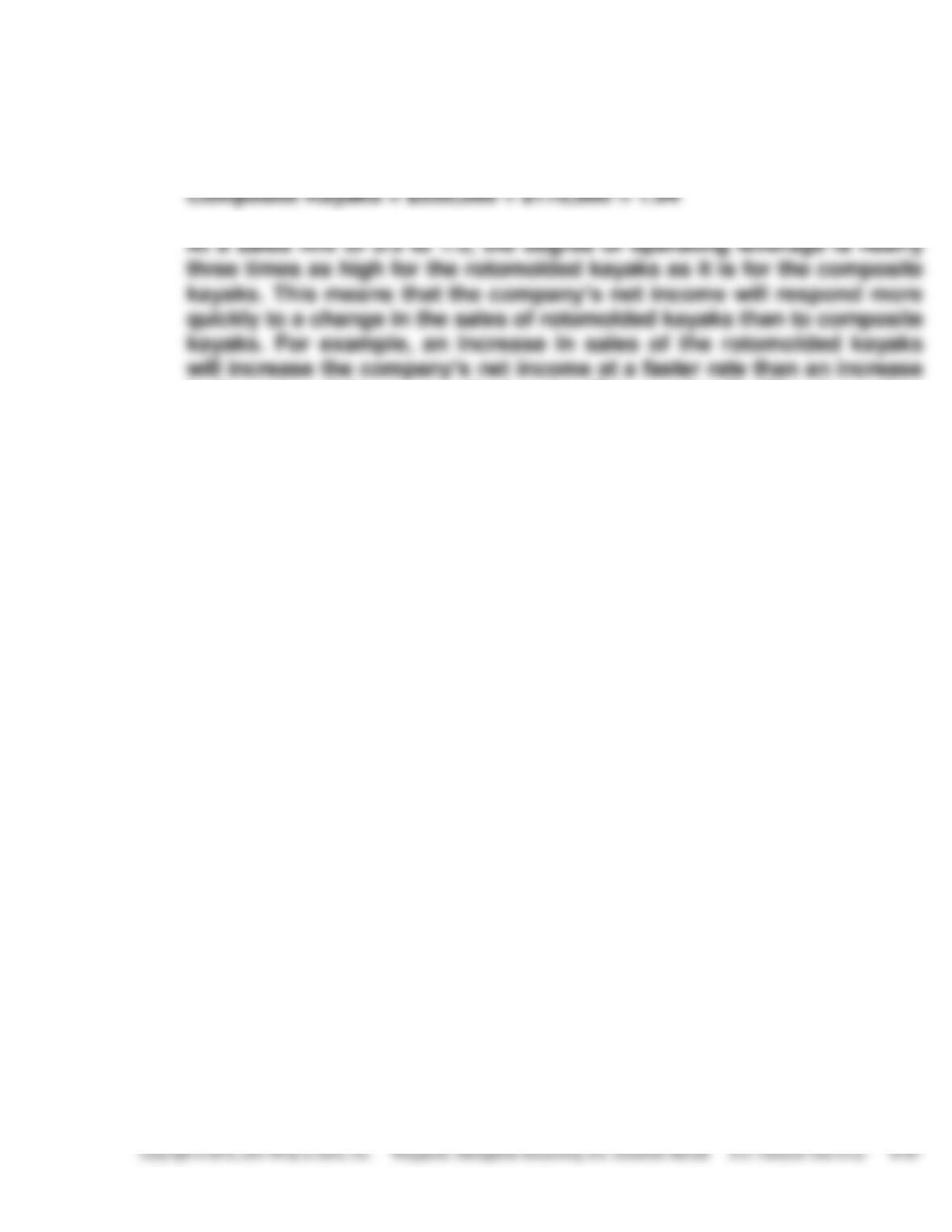
(($950 – $570) X .80)
(($2,000 – $1,340) X .20)
$436
(b) Break-even Sales = $820,000 ÷ $436 = 1,881 units
(c) Target Net Income in Units:
Rotomolded Kayaks
+
Composite Kayaks
=
Weighted-Average
CM/Unit
($380 X .70)
($660 X .30)
$464
Required Sales in Units = ($820,000 + $2,000,000) ÷ $464 = 6,078 units
(d) CVP Income Statement
Rotomolded
Composite
Sales
$2,000,000
$1,000,000
Variable Costs
1,200,000*
670,000**
Contribution Margin
800,000
330,000
Fixed Costs
660,000
160,000
Net Income
$ 140,000
$ 170,000
*($570 ÷ $950) X $2,000,000 **($1,340 ÷ $2,000) X $1,000,000
BYP 6-1 (Continued)
(e) Degree of Operating Leverage
Rotomolded Kayaks = $800,000 ÷ $140,000 = 5.71
in the sales of the composite kayaks. This result will differ depending
on what sales mix assumption is made.
BYP 6-2 DECISION-MAKING ACROSS THE ORGANIZATION
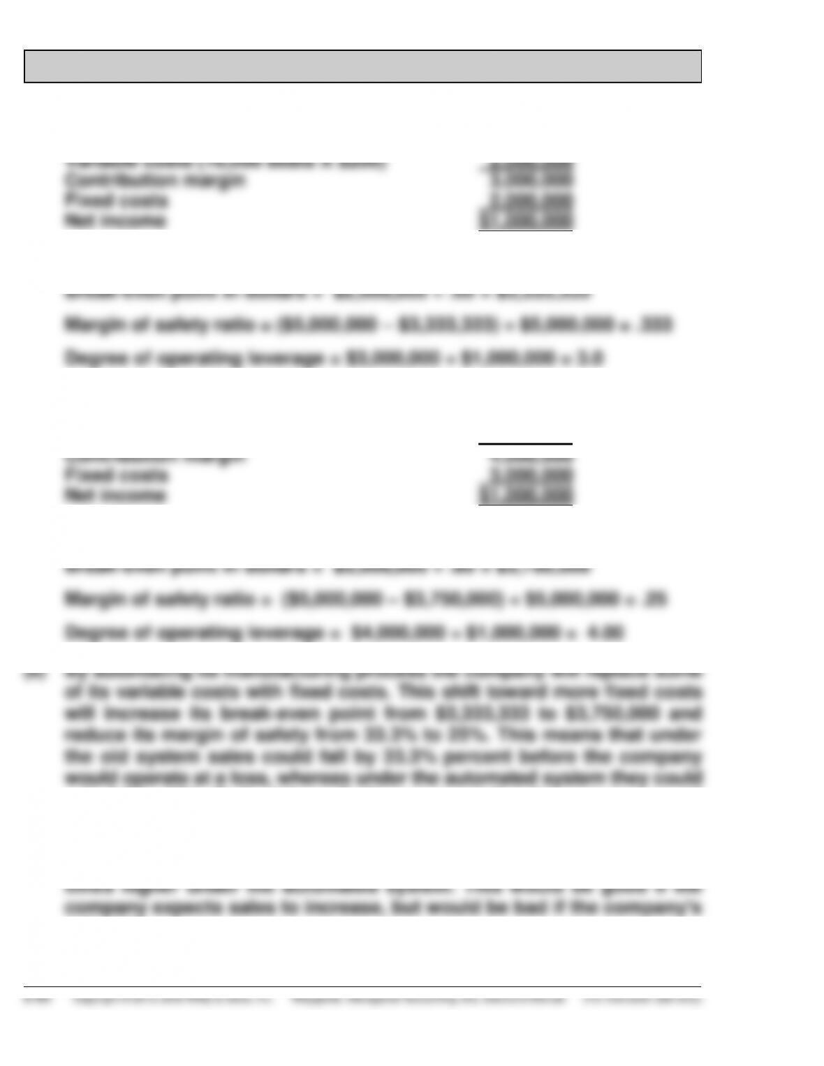
(a)
Sales (10,000 seats X $500) $5,000,000
(b) Contribution margin ratio = $3,000,000 ÷ $5,000,000 = .60
(c)
Sales (10,000 seats X $500) $5,000,000
Variable costs (10,000 seats X $ 100) 1,000,000
(d) Contribution margin ratio = $4,000,000 ÷ $5,000,000 = .80
only fall by 25%. Both of these findings suggest that the company would
be riskier with the automated system. However, the company’s degree
of operating leverage would increase from 3.0 to 4.00. This means that
with a change in sales, the change in net income would be 1.33 (4 ÷ 3)
sales fall.
BYP 6-3 MANAGERIAL ANALYSIS
Current approach $500,000/$2,000,000 = .25
Automated approach $1,000,000/$2,000,000 = .50
This means that for every dollar of sales, net income goes up by
approach.
(b) The break-even points in sales dollars under each approach are:
Current approach $380,000/.25 = $1,520,000
Automated approach $800,000/.50 = $1,600,000
(c) At the current level of sales, the margin of safety ratio under each
approach is:
Current approach ($2,000,000 – $1,520,000)/$2,000,000 = .24
Automated approach ($2,000,000 – $1,600,000)/$2,000,000 = .20
(d) The degree of operating leverage under each approach at the current
level of sales is:
Current approach $500,000/$120,000 = 4.17
Automated approach $1,000,000/$200,000 = 5.00
41.7 percent for the current approach, but 50% for the automated
approach. Recall, however, that at the current level of sales the company
makes considerably more money using the automated approach.