
Case 2
Attiring Situation
Objectives: This case allows the student to create hypotheses and conduct statistical analyses to test
them using data from an experiment.
Summary: RESERV is a national placement firm specializing in putting retailers and service providers
together with potential employees who fill positions at all levels of the organization—from entry-level
positions to senior management positions. One specialty clothing store chain has adopted a very flexible
dress code and is interested in examining if the appearance of potential employees influences customers.
The retailer also is interested in customer integrity. The senior research associate conducts an experiment
to examine relevant research questions including:
RQ1: How does employee appearance affect customer purchasing behavior?
RQ2: How does employee appearance affect customer ethics?
A laboratory experiment is designed in which two variables are manipulated in a between-subjects design:
employee attire (professional/unprofessional) and manner with which the employee tries to gain extra
sales (soft close/hard close). Subjects’ biological sex was recorded and included as a blocking variable.
Four dependent variables are included: TIME (0-10 minutes), SPEND ($0-$25), and KEEP ($0-$25).
Additionally, several variables were collected following the experiment that tried to capture how the
subject felt during the exercise. All of these items were gathered using a 7-item semantic differential
scale.
The experiment was conducted in a university union, and subjects were recruited to participate as
customers who had just purchased some dress slacks and a shirt in a mock retail environment. The
employee was to complete the transaction and try to sell the customer some of several accessory items
displayed at the counter. Each subject was randomly assigned to one of four conditions where the
employee was either:
1. Dressed professionally and used a soft close.
2. Dressed unprofessionally and used a soft close.
3. Dress professionally and used a hard close.
4. Dress unprofessionally and used a hard close.
The researcher wishes to use this information to explain how employee appearance encourages shoppers
to continue shopping (TIME) and spend money (SPEND). Each subject was given $25 (in one-dollar
bills) which they were allowed to spend on accessories. Subjects were not told what to do with any of the
money they did not spend, so the other dependent variable, KEEP, measured how much of the money a
subject kept after returning the questionnaire.
Questions
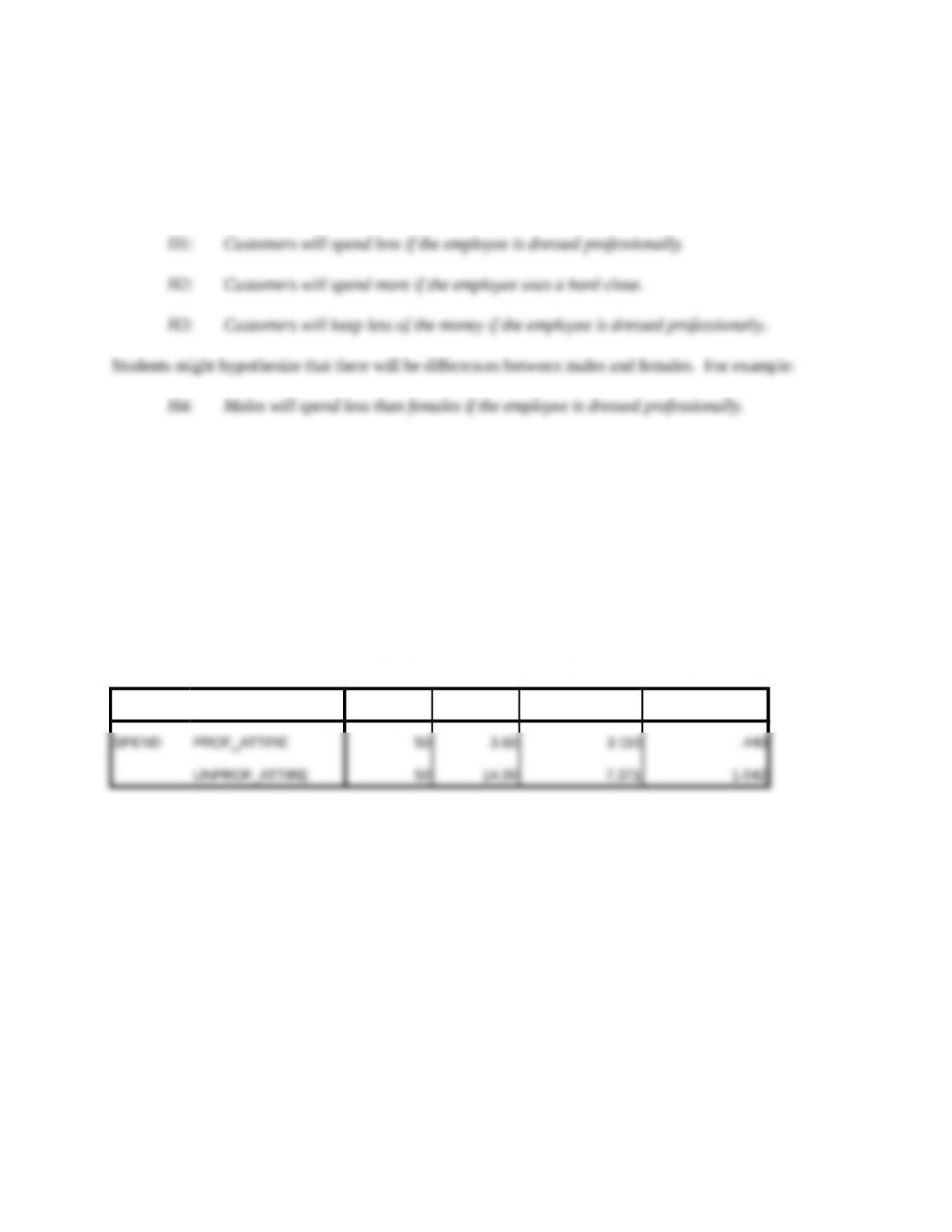
1. Develop at least three hypotheses that correspond to the research questions.
Students’ hypotheses will vary. However, some possible hypotheses are:
Ideally, hypotheses would be developed based on theory or a proposed model that would logically lead to
a specific hypothesis.
2. Test the hypotheses using an appropriate statistical approach.
The appropriate statistical approach will depend on the hypotheses students develop. ANOVA is the
appropriate statistical approach for the hypotheses given above.
To test H1 above, ANOVA is appropriate:
Group Statistics
X1 N Mean Std. Deviation Std. Error Mean
These results suggest that customers spend less when the employee is dressed professionally, providing
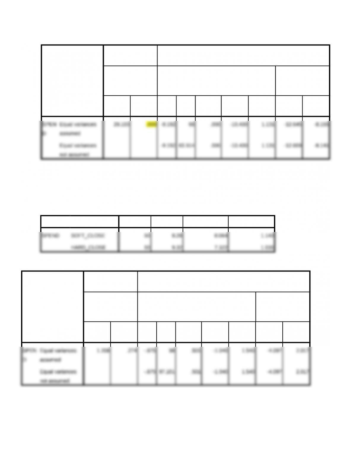
support for H1. However, there is no significant different on the amount spend due to the type of close
used by the employee (H2):
Group Statistics
X2 N Mean Std. Deviation Std. Error Mean
Independent Samples Test
Levene’s Test for
Equality of Variances t-test for Equality of Means
95% Confidence
Interval of the
Difference
F Sig. t df
Sig.
(2-tailed)
Mean
Difference
Std. Error
Difference Lower Upper
not assumed
Independent Samples Test
Levene’s Test for
Equality of Variances t-test for Equality of Means
95% Confidence
Interval of the
Difference
F Sig. t df
Sig.
(2-tailed)
Mean
Difference
Std. Error
Difference Lower Upper
not assumed
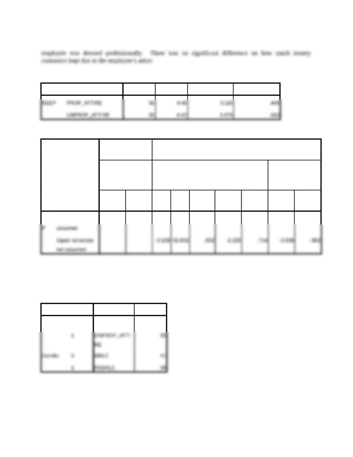
Similarly, the results do not support H3, which hypothesized that customers would keep less money if the
Group Statistics
X1 N Mean Std. Deviation Std. Error Mean
Independent Samples Test
Levene’s Test for
Equality of Variances t-test for Equality of Means
95% Confidence
Interval of the
Difference
F Sig. t df
Sig.
(2-tailed)
Mean
Difference
Std. Error
Difference Lower Upper
KEE
Equal variances
2.735 .101 -3.108 98 .002 -2.220 .714 -3.637 -.803
not assumed
Finally, H4 stated that males would spend less than females if the employee was dressed professionally,
which is supported by the results given below:
Between-Subjects Factors
Value Label N
X1 0 PROF_ATTIRE 50
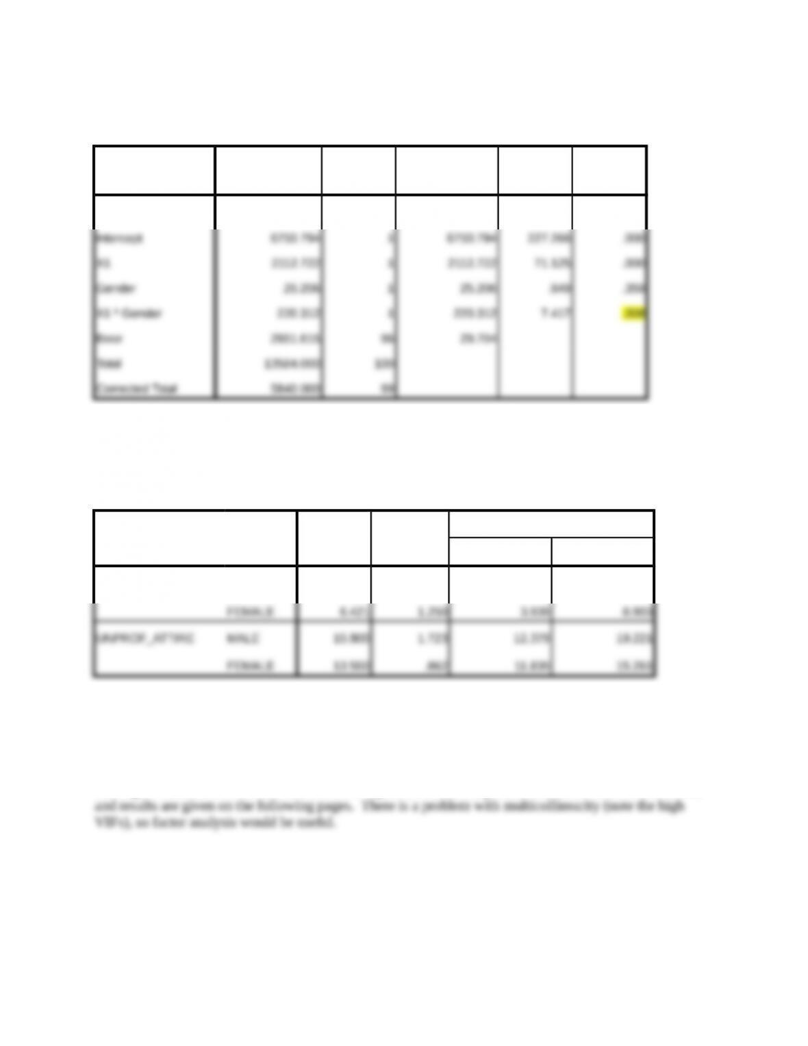
Tests of Between-Subjects Effects
Dependent Variable:SPEND
Source
Type III Sum of
Squares df Mean Square F Sig.
Corrected Model 2988.385a3 996.128 33.535 .000
a. R Squared = .512 (Adjusted R Squared = .496)
EXP1 * Gender
Dependent Variable:SPEND
EXP1 Gender Mean Std. Error
95% Confidence Interval
Lower Bound Upper Bound
PROF_ATTIRE MALE 1.871 .979 -.072 3.814
3. Suppose the researcher is curious about how the feelings captured with the semantic differentials
influence the dependent variables SPEND and KEEP. Conduct an analysis to explore this possibility.
Are any problems present in testing this?
The eight semantic differential variables were regressed on each dependent variable: SPEND and KEEP,
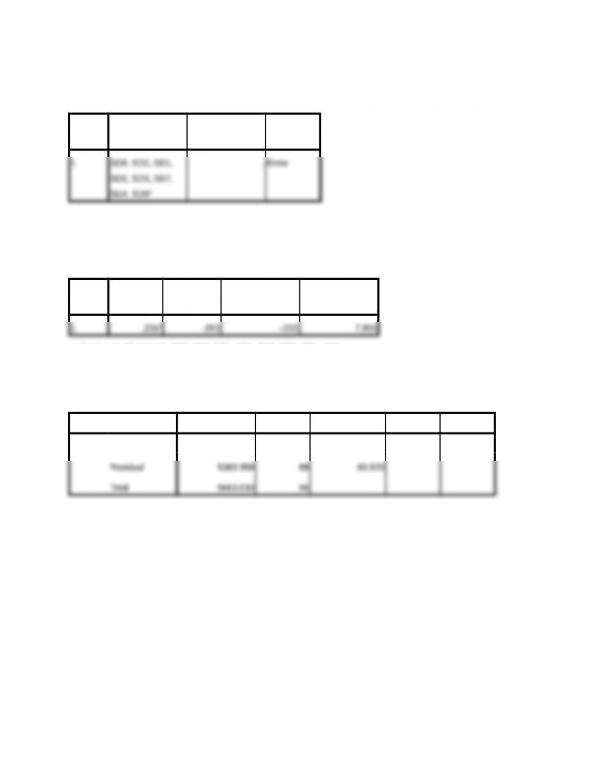
Dependent variable = SPEND, model is not significant (F = 0.62, p = 0.759):
Variables Entered/Removed
Model Variables Entered
Variables
Removed Method
a. All requested variables entered.
Model Summary
Model R R Square Adjusted R Square
Std. Error of the
Estimate
a. Predictors: (Constant), SD8, SD2, SD1, SD5, SD3, SD7, SD4, SD6
ANOVAb
Model Sum of Squares df Mean Square F Sig.
1 Regression 302.072 8 37.759 .620 .759a
a. Predictors: (Constant), SD8, SD2, SD1, SD5, SD3, SD7, SD4, SD6
b. Dependent Variable: SPEND
Coefficientsa
Model
Unstandardized Coefficients
Standardized
Coefficients
t Sig.
Collinearity Statistics
B Std. Error Beta Tolerance VIF
1 (Constant) 39.430 15.430 2.555 .012
SD1 .441 .436 .117 1.012 .314 .809 1.236
SD2 -.067 .718 -.018 -.094 .926 .289 3.456
a. Dependent Variable: SPEND
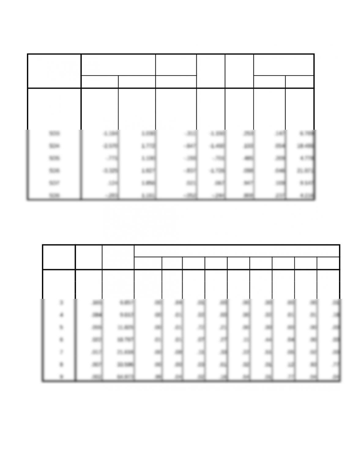
Collinearity Diagnosticsa
Model
Dime
nsion
Eigenvalu
e
Condition
Index
Variance Proportions
(Constant) SD1 SD2 SD3 SD4 SD5 SD6 SD7 SD8
1 1 7.750 1.000 .00 .00 .00 .00 .00 .00 .00 .00 .00
2 .899 2.936 .00 .00 .01 .01 .00 .00 .00 .00 .00
a. Dependent Variable: SPEND
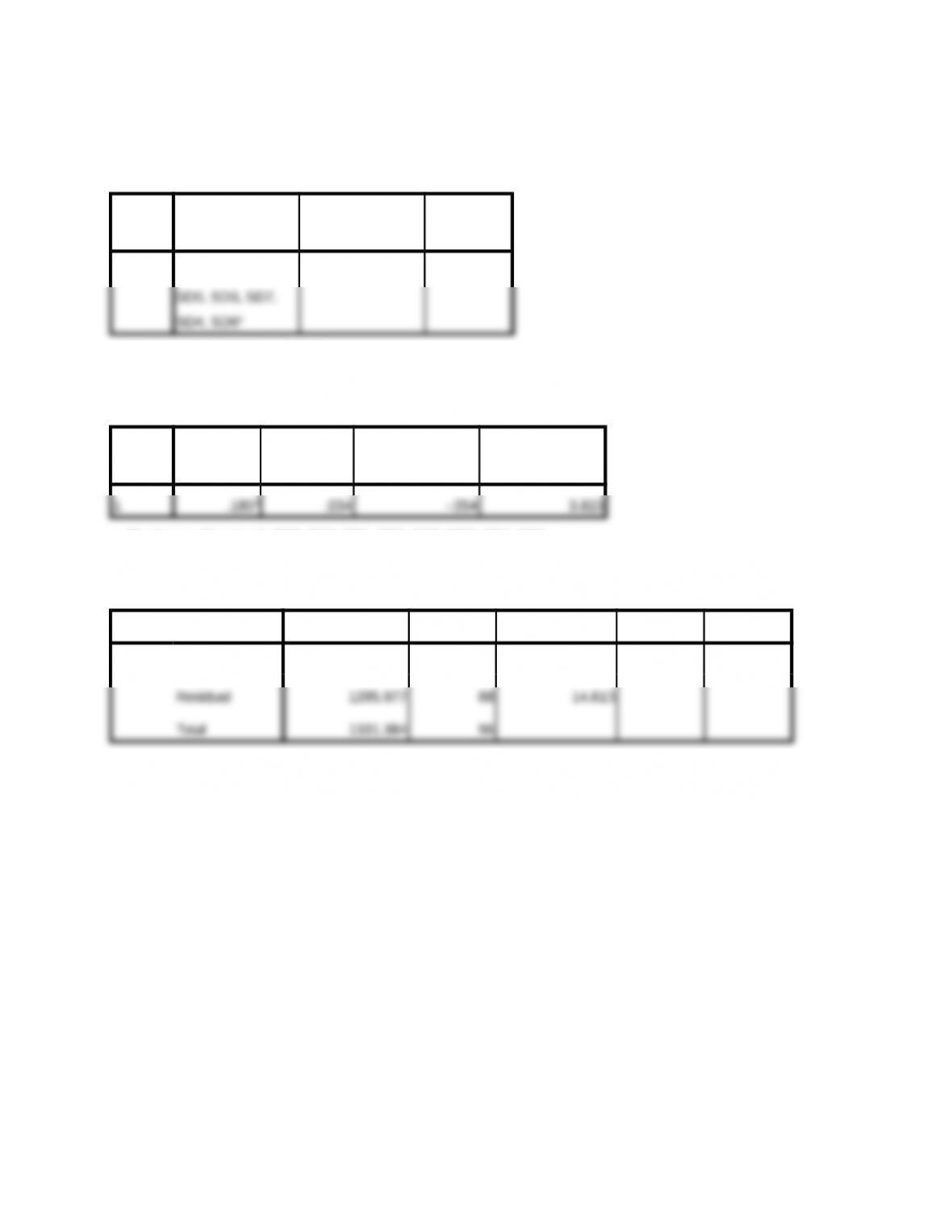
Dependent variable = KEEP, also not significant (F = 0.388, p = 0.924):
Variables Entered/Removed
Model Variables Entered
Variables
Removed Method
1 SD8, SD2, SD1,
. Enter
a. All requested variables entered.
Model Summary
Model R R Square Adjusted R Square
Std. Error of the
Estimate
a. Predictors: (Constant), SD8, SD2, SD1, SD5, SD3, SD7, SD4, SD6
ANOVAb
Model Sum of Squares df Mean Square F Sig.
1 Regression 45.408 8 5.676 .388 .924a
a. Predictors: (Constant), SD8, SD2, SD1, SD5, SD3, SD7, SD4, SD6
b. Dependent Variable: KEEP
Coefficientsa
Model
Unstandardized Coefficients
Standardized
Coefficients
t Sig.
Collinearity Statistics
B Std. Error Beta Tolerance VIF
1 (Constant) 10.477 7.557 1.386 .169
SD1 .072 .213 .039 .336 .737 .809 1.236
a. Dependent Variable: KEEP
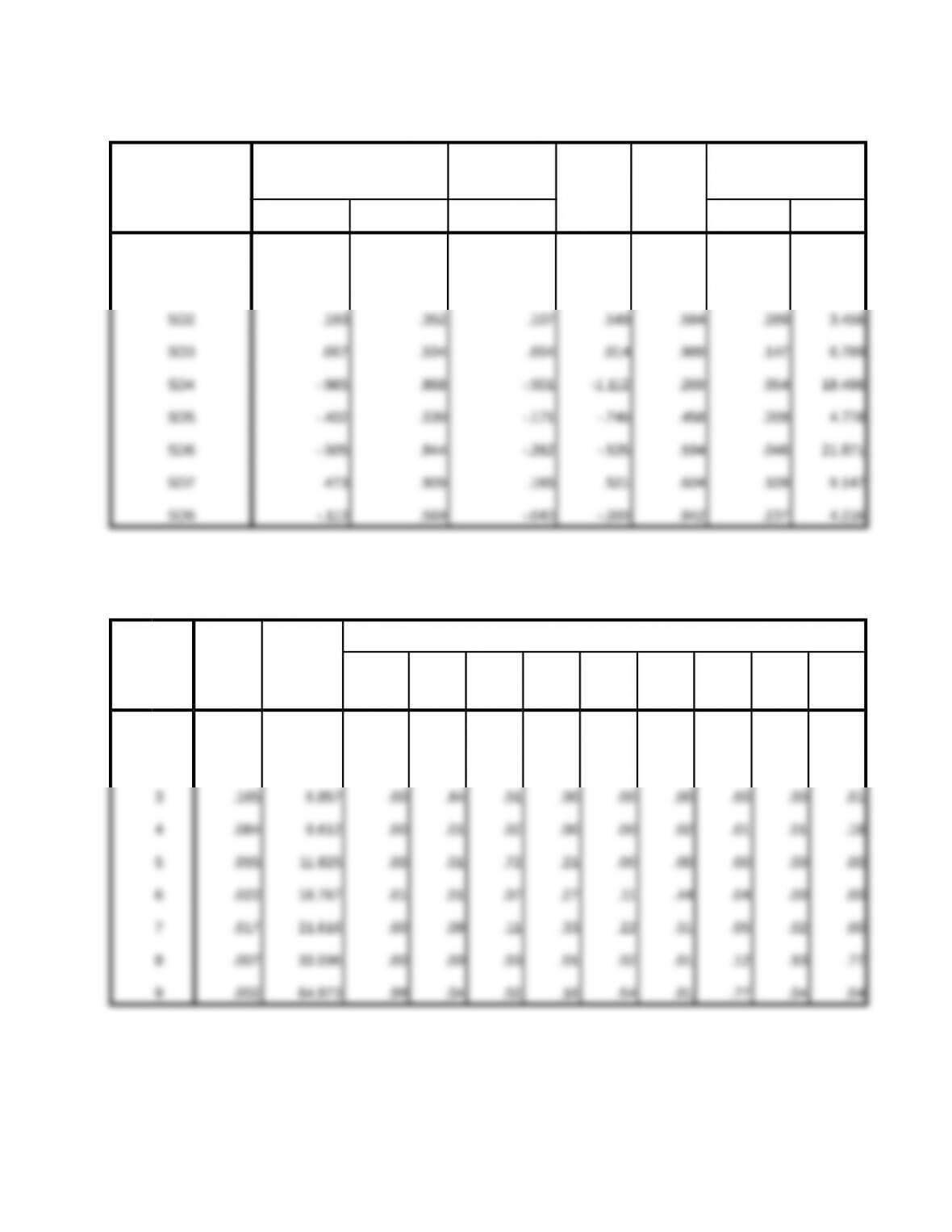
Collinearity Diagnosticsa
Mode
l
Dime
nsion
Eigenvalu
e
Condition
Index
Variance Proportions
(Constant
) SD1 SD2 SD3 SD4 SD5 SD6 SD7 SD8
1 1 7.750 1.000 .00 .00 .00 .00 .00 .00 .00 .00 .00
2 .899 2.936 .00 .00 .01 .01 .00 .00 .00 .00 .00
a. Dependent Variable: KEEP