
Partial differential equations 463
and the ratio is
Qr
2
TrZ1
1/2 dθ2
∂˜y!˜y=L
The Matlab script for this problem is:
1function s13c12p3
2clc
3close all
9nx = 32; %number of nodes in x
10 Tr = 1; %hot temperature on the right
11
12 %make the flux calculations
23 h = figure;
24 plot(T,plot1,‘-or’,T,plot2,‘-ob’)
25 legend(‘Material 1’,‘Material 2’)
26 xlabel(‘Temperature ratio, $T r$‘,‘FontSize’,12)
27 ylabel(‘$Q {numerical}/ Q {resistor}$’,‘FontSize’,12)
38 %set space for the equations in both domains
39 neqs = 2*n;
40 A = zeros(neqs);
41 b = zeros(neqs,1);
42
50 A(edge,edge) = 1; b(edge,1) = 1; %sets temperature to 1
51 %loop over each of the rows
52 for j = 2:ny-1
53 %go down the column
54 r = ny*(i-1) + j; %current location of node
65 %write the first column in the material
66 r = 1;
67 A(r,r) = 1; b(r,1) = 1; %sets temperature to zero
68 for j = 2:ny-1
69 r = j;
are the same as
80 %for the material 1 domain except that everything has to be …
increased by n
81 %= nx*ny
82
92 A(r,r) = -4; %current node
93 A(r,r+1) = 1; %node below
94 A(r,r+ny) = 1; %node to right
95 end
96 edge = n + ny*i; %location of lower edge
105 A(r,r-1) = 1; %node above
106 A(r,r) = -4; %current node
107 A(r,r+1) = 1; %node below
108 A(r,r-ny) = 2; %node to left, includes fictitious node
109 end
118
119 r = n; %bottom node, material 1
120 A(r,r) = 1; %sets temperature = 0
121 r=n+ny;%bottom node, material 2
122 A(r,r) = 1; %sets temperature = 0
131 %use backward differences for material 1
132 A(rtwo,rone-ny) = -k; A(rtwo,rone) = k; %k*dT/dx for …
material 1
133 %use forward differences for material 2 but remember – …
sign in equation
142 h = ny;
143 Tplot = zeros(w,h); %we don’t need to plot the interface twice
144
145 %get out the temperatures in material 1 and the interface
146 for i = 1:nx
156 for j = 1:ny
157 r = (i-1)*ny + j; %node location in material 2
158 Tplot(i-1,j) = Tline(r); %need to shift i-1 for the …
interface
159 end
170 flux2 = (2*L/Tr)*booles(q2,0.5); %0.5 for length of interval
171
172 out = [flux1,flux2];
173
174 function out = booles(q,L)
1 1.5 2 2.5
0.75
0.8
0.85
0.9
0.95
1
1.05
1.1
1.15
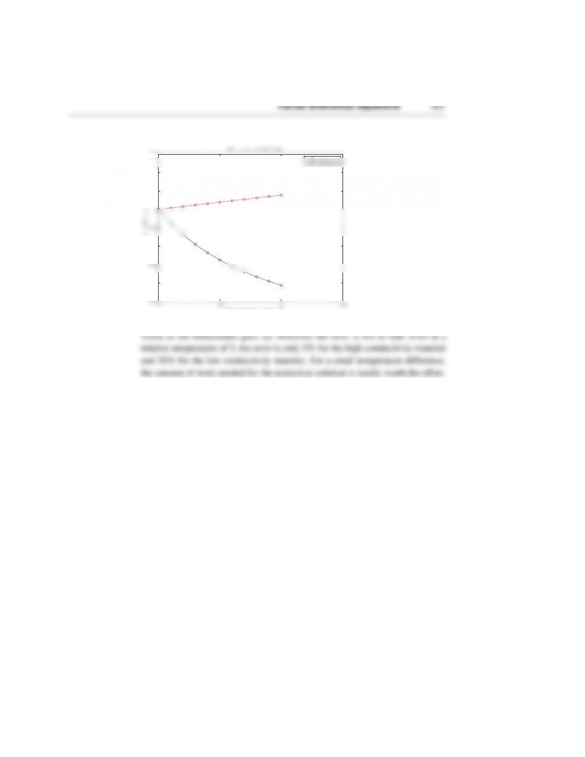
Te m p e ra tu r e r at i o , Tr
Qn u m e r i c a l
/Q r e s i s t o r
S ol u ti o n t o s 13 c 12p 3
M a t e r i a l 1
M a t e r i a l 2
The resistor model is best for the high conductivity material, and the model gets

8Interpolation and integration
476 Interpolation and integration
Problems
(8.1) 4 points
(8.2) The recursion relationship gives
We already have a result for the third-order divided-differences so we can use that
(8.3) For n=6, we would like to approximate the integral as
I=Zx0+6h
x0
f6(x)+R6dx
If we convert into the form with α, then we have
I=hZ6
f6(α)+R6dα
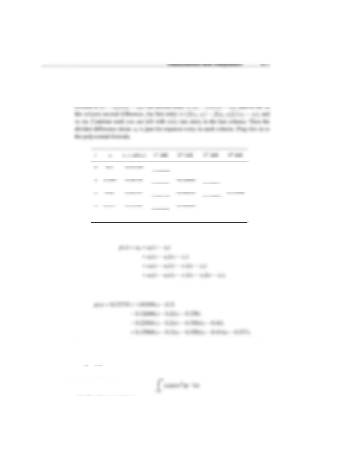
(8.4) The divided difference formula is recursive. In the table below, the differences are
generated from the previous column. E.g., the first entry under the first difference
1.04209
0.97346 -0.22981
0.90110 -0.16594
0.81667
4 0.6 0.60386
The interpolating polynomial is:
where a0=y0,a1=1st difference, a2=2nddifference, a3=3rd difference, and
a4=4th difference. Plugging in the values from the table above,
Evaluating p(x) at x=0.5, p(0.5) =0.52050. The Matlab output for erf(0.5) is
0.5204998 . . .. Considering that we rounded offat 5 decimal places, the agreement is
very good.
(8.5) x=1
2±1
2√3
(8.6) (a) The problem is
0
(b) Romberg integration
(c) nis the number of trapezoids for the lowest order (first) integral
(d) multiple trapezoidal rule

(8.7) The files for this problem are contained in s15c7p2 matlab.
The program is:
1function s15h7p2
2clc
3close all
14
15 %make the plot of the function
16 yexact = zeros(1,nplot);
17 for i = 1:nplot
18 yexact(i) = getf(xplot(i));
\n’,i-1,coeff(i),i-1,x(i))
29 end
30 fprintf(‘\n’)
31
32 %make the plot
43 legend boxoff
44 xlabel(‘$x$’,‘FontSize’,14)
45 ylabel(‘$f(x)$’,‘FontSize’,14)

Interpolation and integration 479
46 saveas(g,‘s15h7p2 solution fig1.eps’,‘psc2’)
57 % x = value of x to interpolate y
58 % xpts = interpolation points
59 % coeffs = interpolation coefficients
60 % n = power of interpolant
61
72 out = y;
73
74
75 function [x,coeff] = integrate interpolation equal(xmin,xmax,n)
76 %xmin = lowest interpolation point
86 U(i,1) = (getf(x(i+1)) – getf(x(i)))/h;
87 end
88
89 %compute higher-order divided differences
90 for j = 2:n
480 Interpolation and integration
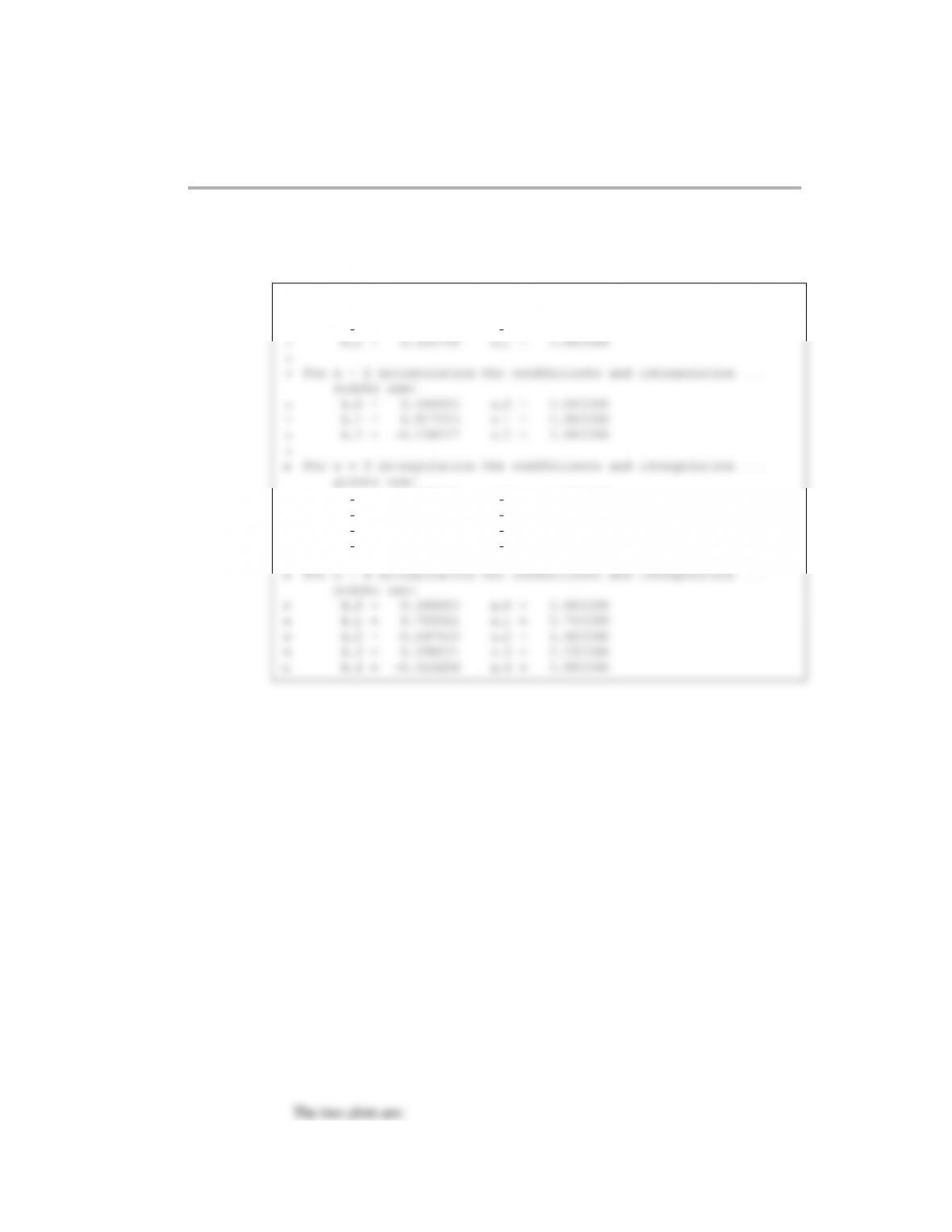
The text output of the program is
1For n = 1 interpolation the coefficients and interpolation …
points are:
2b 0 = 0.000000 x 0 = 0.000000
11 b 0 = 0.000000 x 0 = 0.000000
12 b 1 = 0.632121 x 1 = 1.000000
13 b 2 = -0.199788 x 2 = 2.000000
14 b 3 = 0.042097 x 3 = 3.000000
15
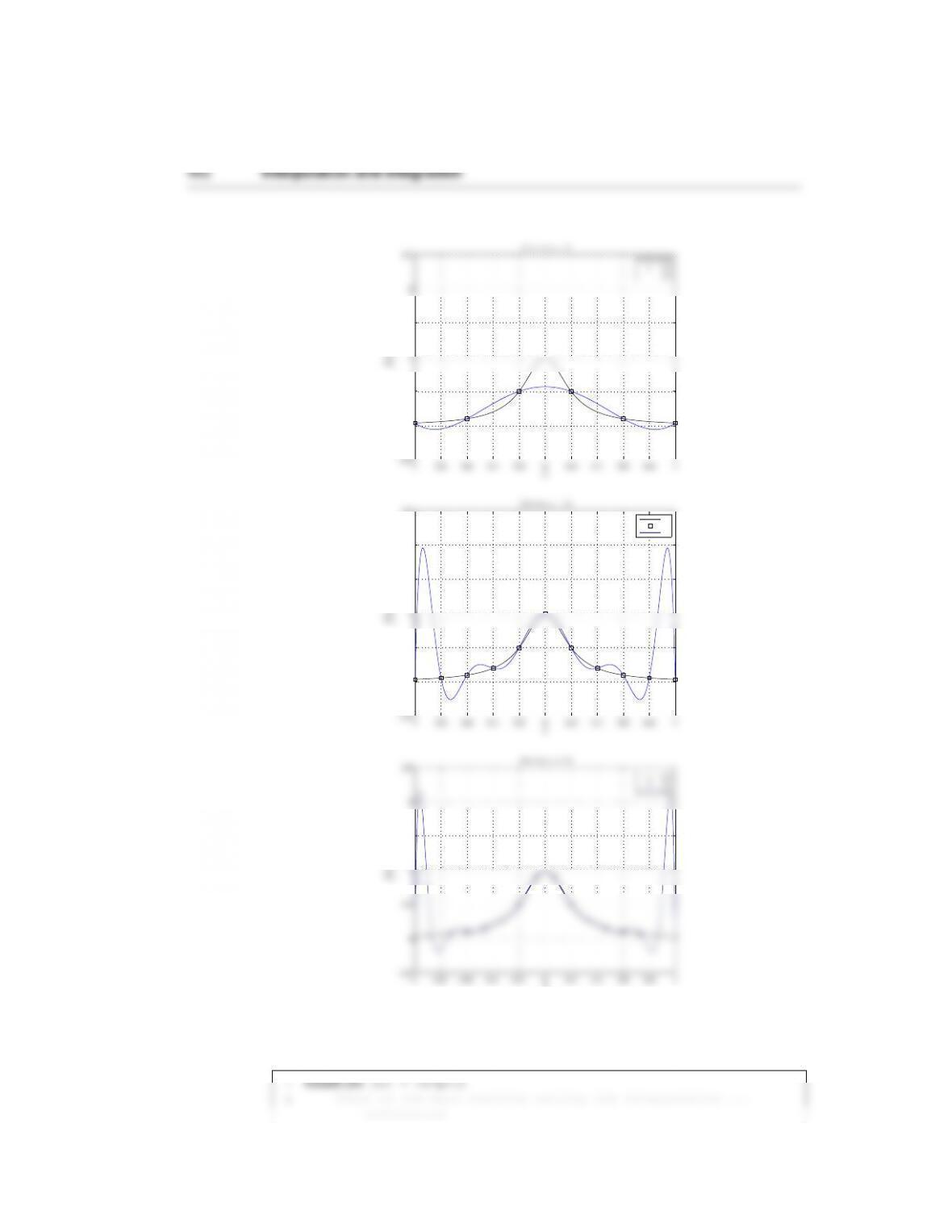
9x tilde = linspace(-1.0, 1.0, 500);
10 y tilde = f(x tilde);
11
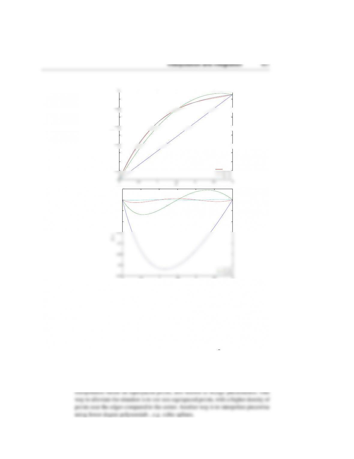
12 %Interpolate different degrees on polynomials
13 for n = 5:5:15
24 title([‘Plot for n = ‘, num2str(n)])
25 xlabel(‘$x$’,‘FontSize’, 14)
26 ylabel(‘$f(x)$’,‘FontSize’, 14)
27 grid on
28 end
38 poly coeff = zeros(Npts, 1);
39 alpha cumprod = zeros(Npts, 1);
40 Neval = length(X tilde);
41 Y hat = zeros(Neval,1);
42
53 for i = 1:Neval
54 alpha = ( X tilde(i) – X(1) )/h;
55
56 %Calculate the vector of cumulative product of alpha
57 alpha cumprod(1) = 1;

66 end
67 end
68
69 %Subfunction to evaluate f(x).
70 %Input: vector X
(8.9) The files for this problem are contained in s15c7p3 matlab.
The program is:
1function s15h7p3
2clc
3close all
14 n(i) = i;
15 I(i) = integrate multiple trapezoidal(xmin,xmax,i);
16 end
17
18 g = figure;
29 I = getf(xmin) + getf(xmax);
30 if n>1
31 for i = 2:n
32 I=I+2*getf(x(i));
33 end


not required
27
28
29 %simpson’s 3/8 rule
30 f = get points(4);
40 fprintf(fid,‘Booles rule: \t\t I = %8.6f\n’,I); %to file, not …
required
41
42
43 %5th order
53 fprintf(’10 trapezoidal rules: \t I = %8.6f\n’,I)
54 fprintf(fid,’10 trapezoidal rules: \t I = %8.6f\n’,I); %to …
file, not required
55
56
66 fprintf(‘Gauss quadrature: \t I = %8.6f\n’,I)
67 fprintf(fid,‘Gauss quadrature: \t I = %8.6f\n’,I); %to file, …
not required
68
69

78 I one = ntrapezoid(10);
79 I two = ntrapezoid(100);
80 I = I two + (I two–I one)/99;
81 fprintf(‘Richardson (10/100): \t I = %8.6f\n’,I)
82 fprintf(fid,‘Richardson (10/100): \t I = %8.6f\n’,I); %to …
91 fsum = f(1) + f(ntraps);
92 for i = 2:ntraps-1
93 fsum = fsum + 2*f(i);
94 end
95 ntraps = ntraps – 1; %remove the extra evaluation point to get …
104 for i = 1:n
105 out(i) = feval(x(i));
106 end
107
108