Partial differential equations 443
ck+n. The new equations for y=0 are
We also need to change the lower corners to no-flux boundary conditions. This
leads to
The no-flux corner boundary condition is discussed in the last recitation.
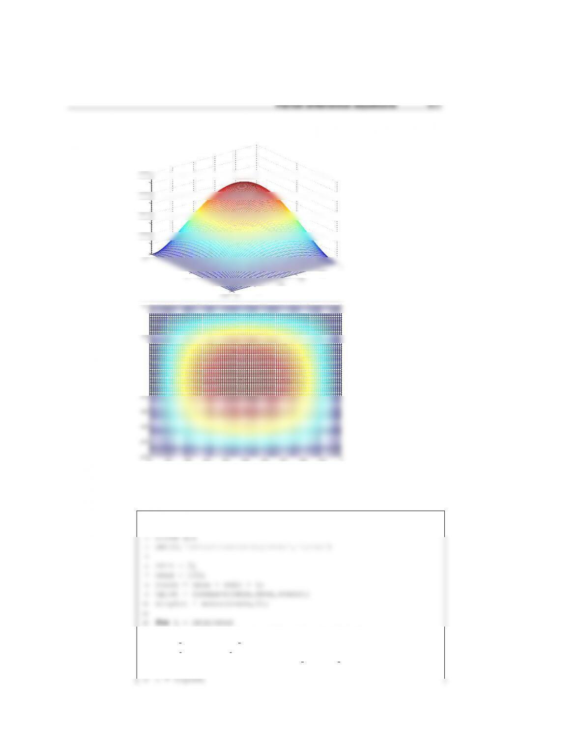
The exact solution is c=1.
The Matlab file for this problem is
1function s15h12p2
2clc
3close all
4set(0,‘defaulttextinterpreter’,‘latex’)
5
6%setup grid
7n = 101;
8dx = 1/(n-1);
9A = zeros(nˆ2);
10 b = zeros(nˆ2,1);
21 end
22 end
23
24 %bottom nodes
25 i = 1;
36 i = n;
37 for j = 2:n-1
38 k = (i-1)*n + j;
39 A(k,k) = 1;
444 Partial differential equations
50 A(k,k+n) = 1;
51 end
52
53 %right nodes
54 j = n;
65 A(n,n) = -2; A(n,n-1) = 1; A(n,2*n) = 1; b(n) = 0;
66 A((n-1)*n+1,(n-1)*n+1) = 1; b((n-1)*n+1) = 1;
67 A(nˆ2,nˆ2) = 1; b(nˆ2) = 1;
68
69 %solve
80 c(i,j) = xsolve(k);
81 x(i,j) = (j-1)*dx;
82 y(i,j) = (i-1)*dx;
83 end
84 end
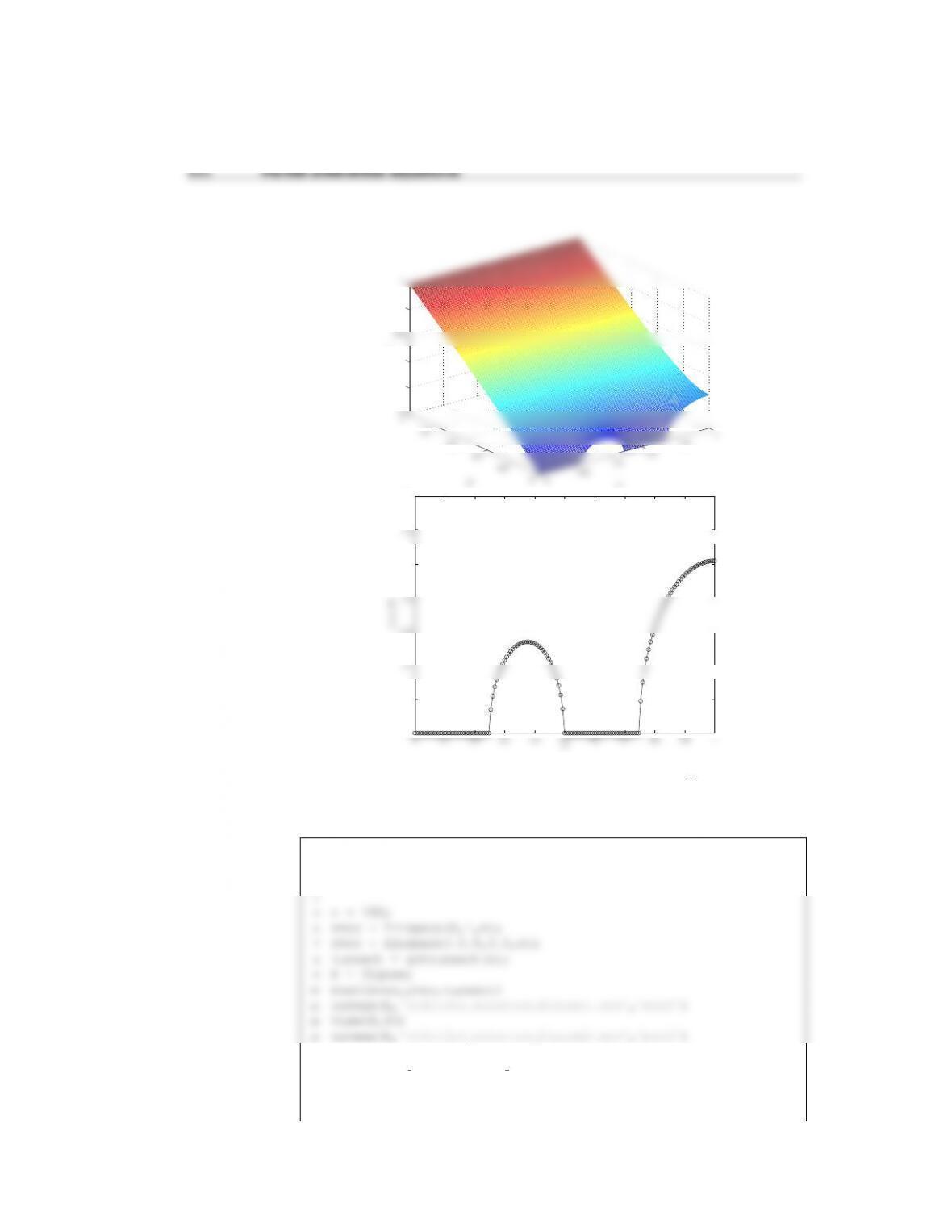
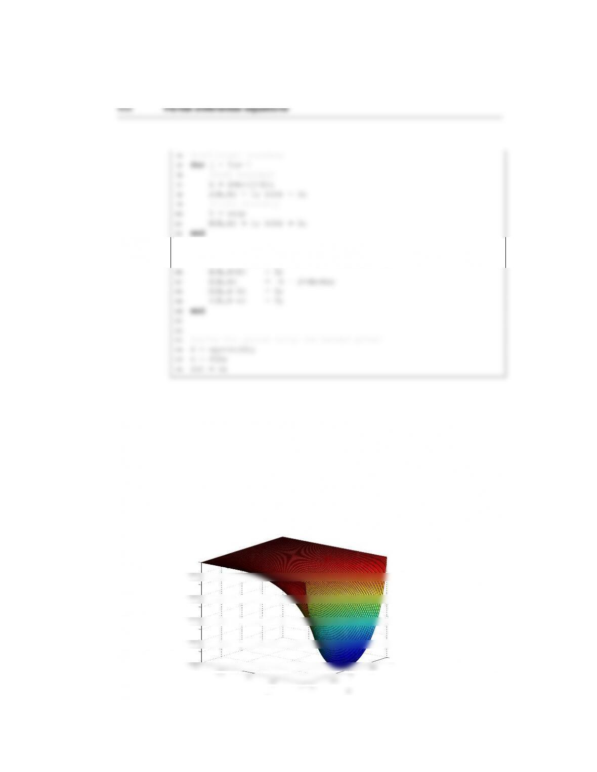
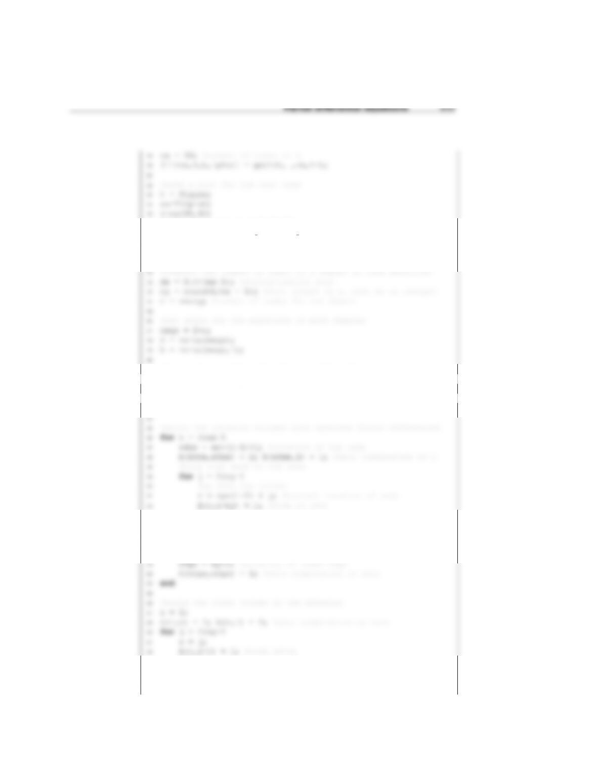
95 %plot the concentration
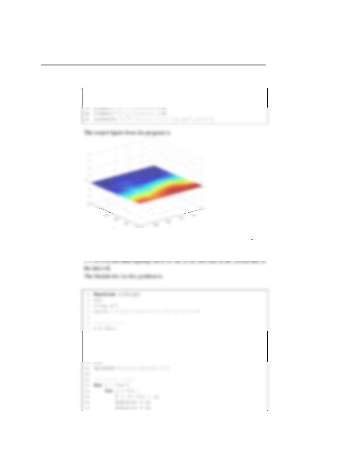
Partial differential equations 445
96 h = figure;
97 mesh(x,y,c)
98 xlabel(‘$x$’,‘FontSize’,14)
0
0.2
0.4
0.6
0.8
1
0
0.2
0.4
0.6
0.8
1
1
1
1
1
1
1
1
1
x
y
c
(c) The files for solving this problem are contained in the directory s15c12p3 matlab
The only change is to use the right boundary conditions on the bottom. This is
implemented by using the mod function to map the x-position back to the interval
8dx = 1/(n-1);
9A = zeros(nˆ2);
10 b = zeros(nˆ2,1);
11 w = 0.5;
12
22 A(k,k) = -4;
23 A(k,k+1) = 1;
24 A(k,k+n) = 1;
25 end
26 end
37 A(k,k+n) = 2;
38 else
39 A(k,k) = 1;
40 b(k) = 0;
41 end
52 %left nodes
53 j = 1;
54 for i = 2:n-1
55 k = (i-1)*n + j;
56 A(k,k-n) = 1;
67 A(k,k-1) = 2;
68 A(k,k) = -4;
69 A(k,k+n) = 1;
70 end
71
81 fprintf(‘Solving matrix.\n’)
82 tic
83 %solve
84 A = sparse(A);
85 xsolve = A\b;
96 c(i,j) = xsolve(k);
97 x(i,j) = (j-1)*dx;
98 y(i,j) = (i-1)*dx;
99 end
100 end
111
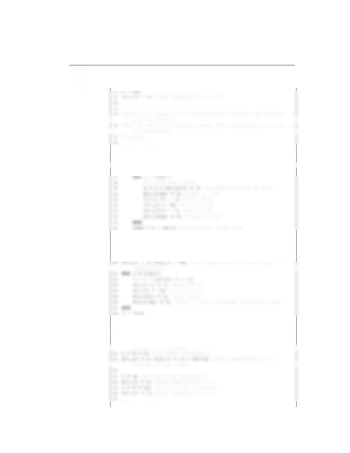
112 %plot the boundary concentration
113 h = figure;
114 plot(x(1,:),c(1,:),‘-ok’)
115 xlabel(‘$x$’,‘FontSize’,14)
cosh(m*pi*y)/cosh(m*pi/2))*sin(m*pi*x);
28 end
29 end
30 end
I have made the plot in the default orientation in Matlab and rotating it so that
0
0.2
0.4
0.6
0.8
1
−0.5
0
0.5
0
0.01
0.02
0.03
0.04
0.05
0.06
0.07
0.08
0 0.1 0.2 0.3 0.4 0.5 0.6 0.7 0.8 0.9 1
−0.5
−0.4
−0.3
−0.2
−0.1
0
0.1
0.2
0.3
0.4
0.5
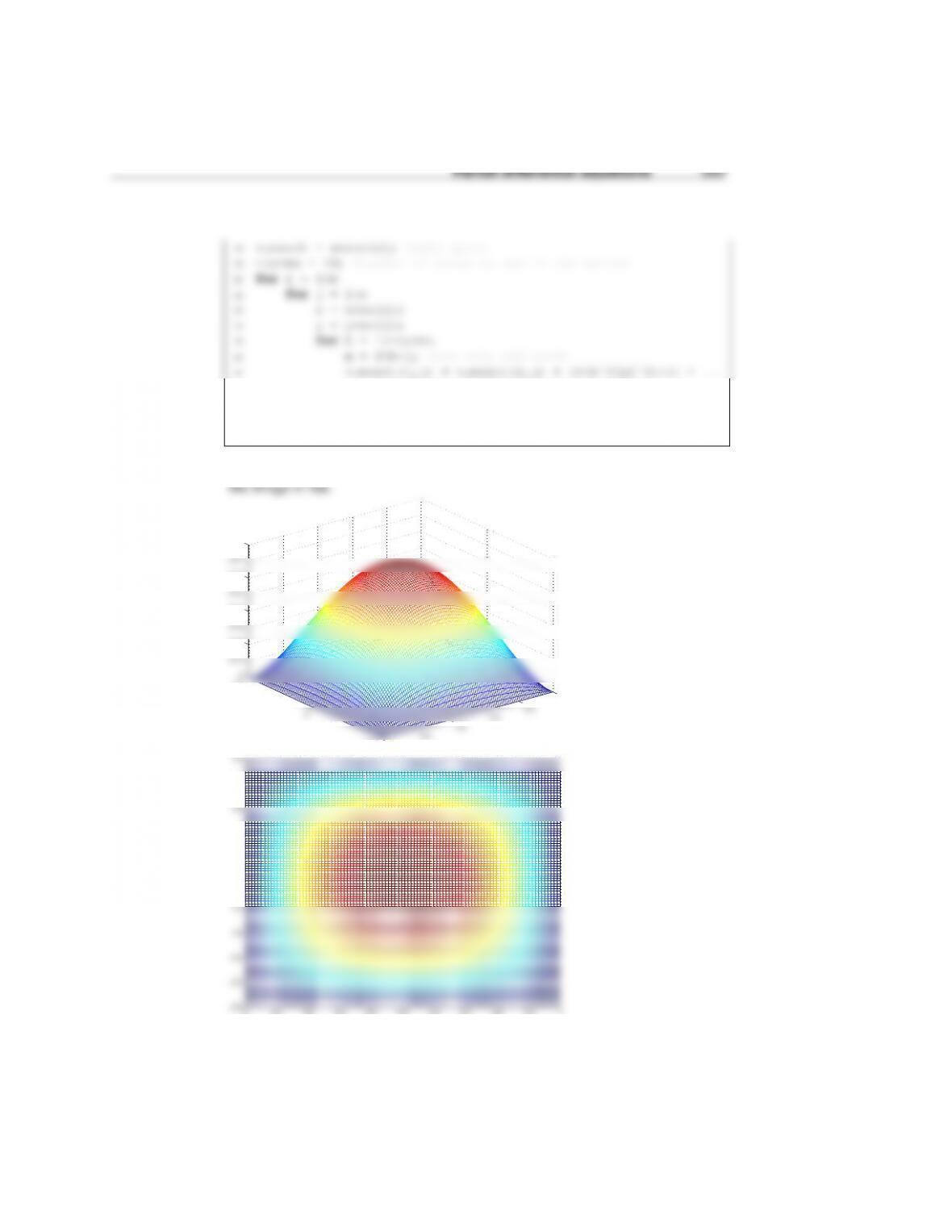
(b) For the interior nodes, using the global counter k, we have
vk−n+vk−1−4vk+vk+1+vk+n=−(∆x)2
while all of the edge nodes have vk=0.
The Matlab program is
450 Partial differential equations
1function s14c12p2
2clc
3close all
11 saveas(h,‘s14c12p2 solution figure1.eps’,‘psc2’)
12 view(0,90)
13 saveas(h,‘s14c12p2 solution figure2.eps’,‘psc2’)
14
25 A(k,k) = -4;
26 A(k,k+1) = 1;
27 A(k,k+n) = 1;
28 b(k) = -dxˆ2;
29 end
40 end
41 for i=n*(n-1)+1:nˆ2
42 A(i,i) = 1; %top of the cell
43 end
44 A = sparse(A); %to use banded solver
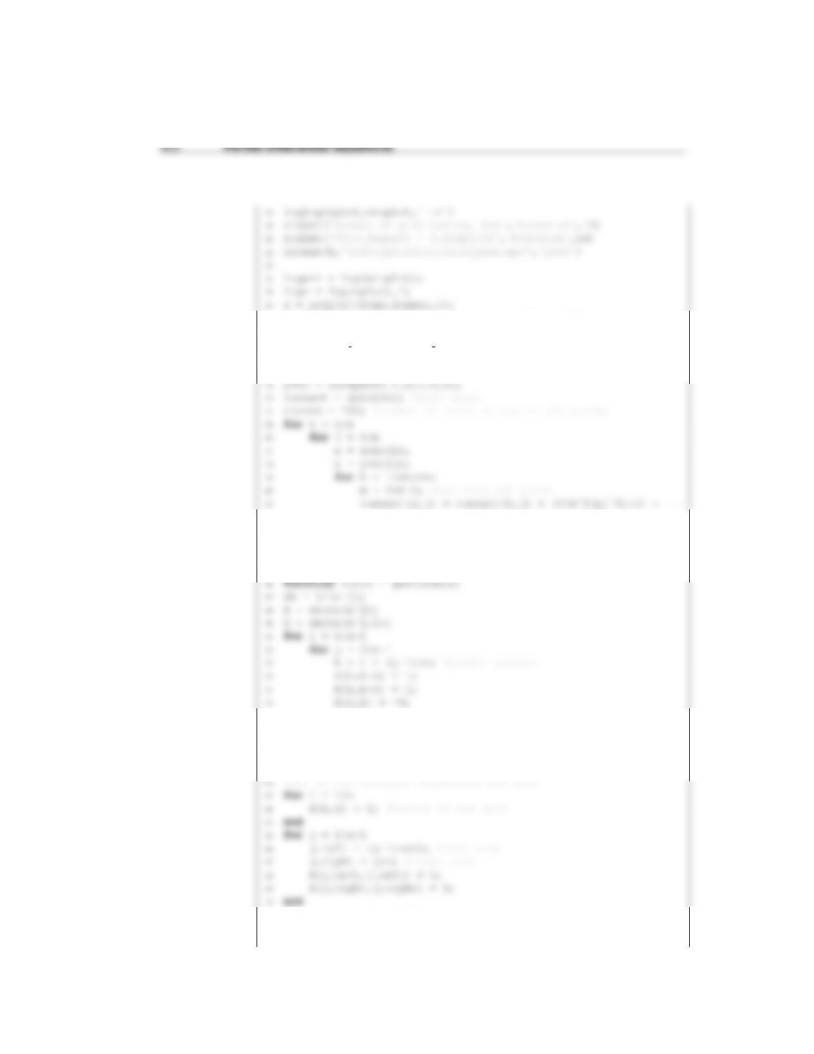
27 fprintf(‘The slope of the line is %6.4f\n’,a(1))
28
29 function v exact = getv exact(n)
30 dx = 1/(n-1);
31 xvec = linspace(0,1,n);
cosh(m*pi*y)/cosh(m*pi/2))*sin(m*pi*x);
42 end
43 end
44 end
45
56 A(k,k+1) = 1;
57 A(k,k+n) = 1;
58 b(k) = -dxˆ2;
59 end
60 end
71 for i=n*(n-1)+1:nˆ2
72 A(i,i) = 1; %top of the cell
73 end
Partial differential equations 453
74 A = sparse(A); %to use banded solver
454 Partial differential equations
Substituting in the differential equation makes the upper boundary have the form
ck+1−[4 +2(∆y)k]ck+ck−1+2ck −n=0
1function s12c12p3
2clc
3close all
4set(0,‘defaulttextinterpreter’,‘latex’)
5
16 for j = 1:n
17 k = i + (j-1)*n;
18 cplot(i,j) = c(k);
19 end
20 end
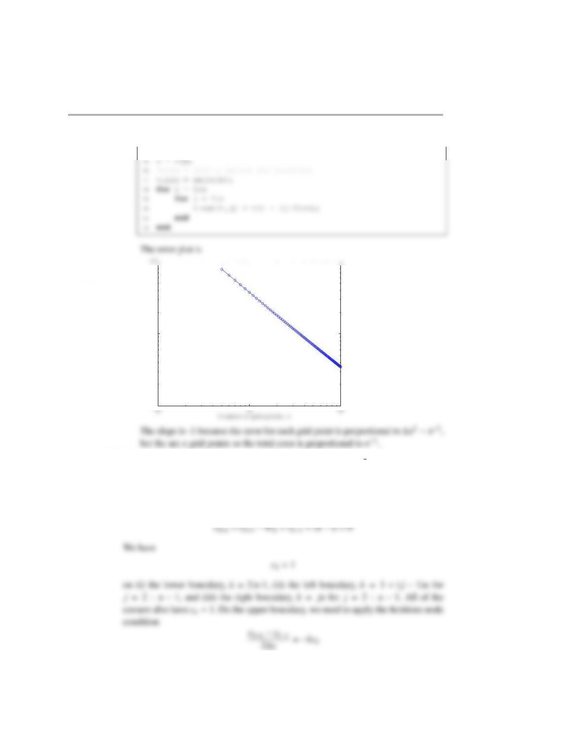
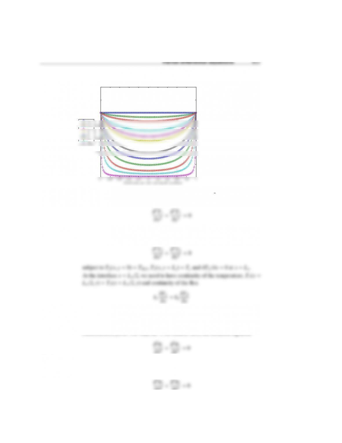
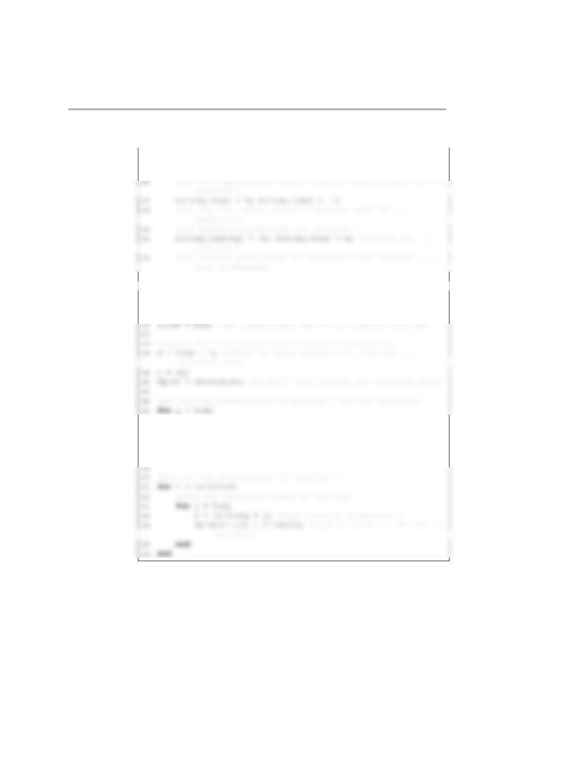
30 %reaction rates
31 csurf = surface c(c,n);
32 plot(x,csurf,‘-ob’)
33
34 kr = [0,0.1,0.2,0.5,0.75,1,2,3,5,10,20,100];
44 xlabel(‘Position on the catalyst surface’,‘FontSize’,14)
45 ylabel(‘Concentration’,‘FontSize’,14)
46 legend(‘0’,‘0.1’,‘0.2’,‘0.5’,‘0.75’,‘1’,‘2’,‘3’,‘5’,’10’,…
47 ’20’,‘100’,‘Location’,‘WestOutside’)
48 saveas(h,‘s12c12p3 solution figure2.eps’,‘psc2’)
59 out = csurf;
60
61
62 function out = compute c(kr,n)
63 %solves the PDE
74 k=i+n*(j-1); %location of node
75 A(k,k+n) = 1;
76 A(k,k+1) = 1;
77 A(k,k) = -4;
78 A(k,k-1) = 1;
89 %lower boundary
90 for k = 2:n-1
91 A(k,k) = 1; b(k) = 1;
92 end
93
103
104 for i = 2:n-1
105 k=i+n*(n-1); %top row, reaction zone
The output files are:
−0.5
0
0.5
1−1
−0.5
0
1
0.55
0.6
0.65
0.7
0.75
0.8
0.85
0.9
0.95
1
x
c
458 Partial differential equations
At the interface ˜x=1/2, we need to have continuity of the temperature, θ1( ˜x=
1/2,˜y)=θ2( ˜x=1/2,˜y) and continuity of the flux
∂˜x
∂˜x
Since the discontinuous boundary condition does not allow for continuity of the
temperature, we will set the temperature at the interface to be the average of the
two temperatures, θ1( ˜x=1/2,˜y=0) =(1 +Tr)/2.
(b) The diffusion equations inside the boundary are
For the top and bottom boundary, the equations are fixed to the constants 1, 0, and
Trdepending on the location. For the left boundary, we need to use the fictitious
node to get
where the subscripts iis the interfacial node in material 1(and we store the tem-
perature condition in that node). For the flux condition, which is stored in the
interface node for material 2, using backward differences gives
where inow refers to the interfacial node for material 2.
The Matlab script of this problem is:
1function s13c12p2
12
13 [Tline,A,b,Tplot] = getT(k,L,nx,Tr);
14 dlmwrite(‘s13c12p2A.dat’,A)
15 dlmwrite(‘s13c1212p2b.dat’,b)
16 dlmwrite(‘s13c12p2T.dat’,Tline)
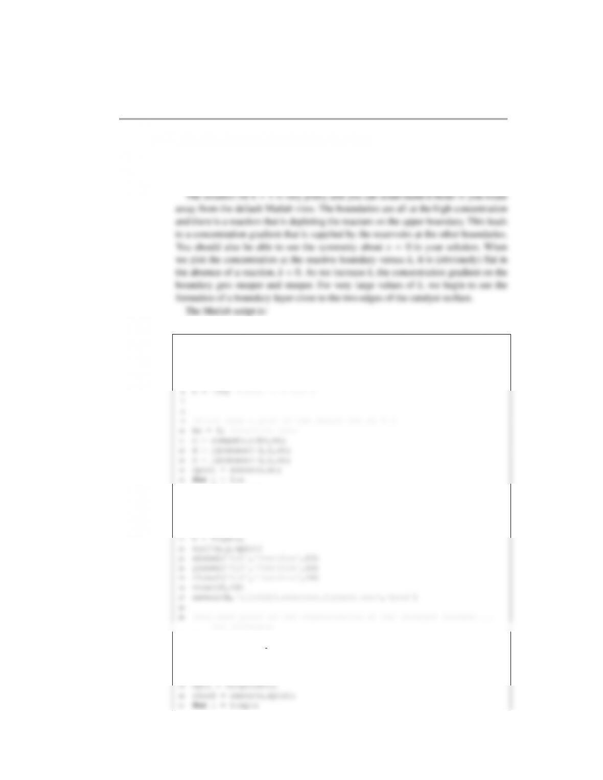
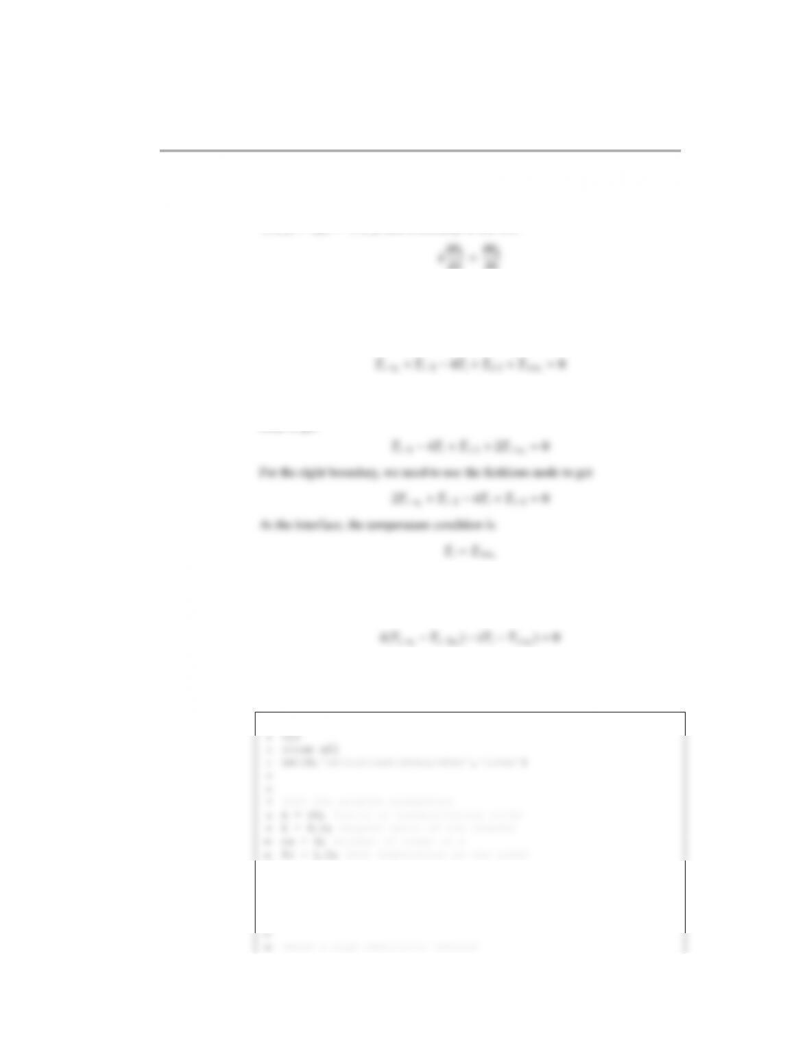
26 title(‘Solution to s13c12p2’)
27 saveas(h,‘s13c12p123 solution figure1.eps’,‘psc2’)
28
29
30 function [Tline,A,b,Tplot] = getT(k,L,nx,Tr)
41 %write the equations for the material 1 domain, starting …
from the upper
42 %left corner and working down in y. This is not the best …
band structure
43 %but easy to write and decompose
54 A(r,r-1) = 1; %node above
55 A(r,r) = -4; %current node
56 A(r,r+1) = 1; %node below
57 A(r,r+ny) = 1; %node to right
58 end
69 A(r,r) = -4; %current node
70 A(r,r+1) = 1; %node below
71 A(r,r+ny) = 2; %node to right, includes fictitious node
72 end
460 Partial differential equations
81 for i = 2:nx-1
82 edge = n + ny*(i-1)+1; %location of top edge
83 A(edge,edge) = 1; b(edge,1) = Tr; %sets temperature to …
hot right temperature
84 %loop over each of the rows
95 A(edge,edge) = 1; %sets temperature to zero
96 end
97
98 %write the last column in the material
99 r=n+ny*(nx-1) + 1;
109 A(r,r) = 1; %sets temperature to zero
110
111 %write the interfacial temperature conditions.
112 r = ny*(nx-1)+1; %top node, material 1
113 A(r,r) = 1; b(r,1) = (1 + Tr)/2; %sets temperature to …
122 for j = 2:ny-1
Partial differential equations 461
123 %loop over the interior nodes
124 rone = ny*(nx-1) + j; %node location in material 1
125 rtwo = n + j; %node location in material 2
132 A(rtwo,rtwo) = 1; A(rtwo,rtwo + ny) = -1; %-dT/dx for …
material 2
133 end
134
135 %solve the system
145 for j = 1:ny
146 r = (i-1)*ny + j; %node location
147 Tplot(i,j) = Tline(r);
148 end
149 end
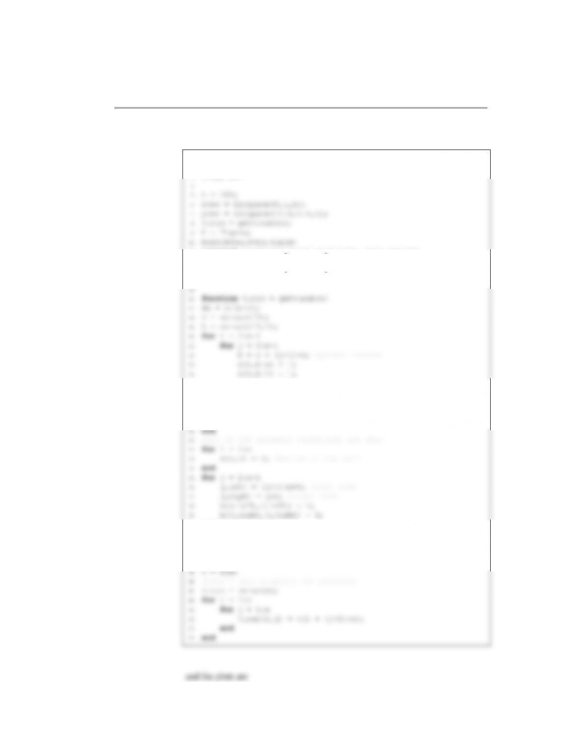
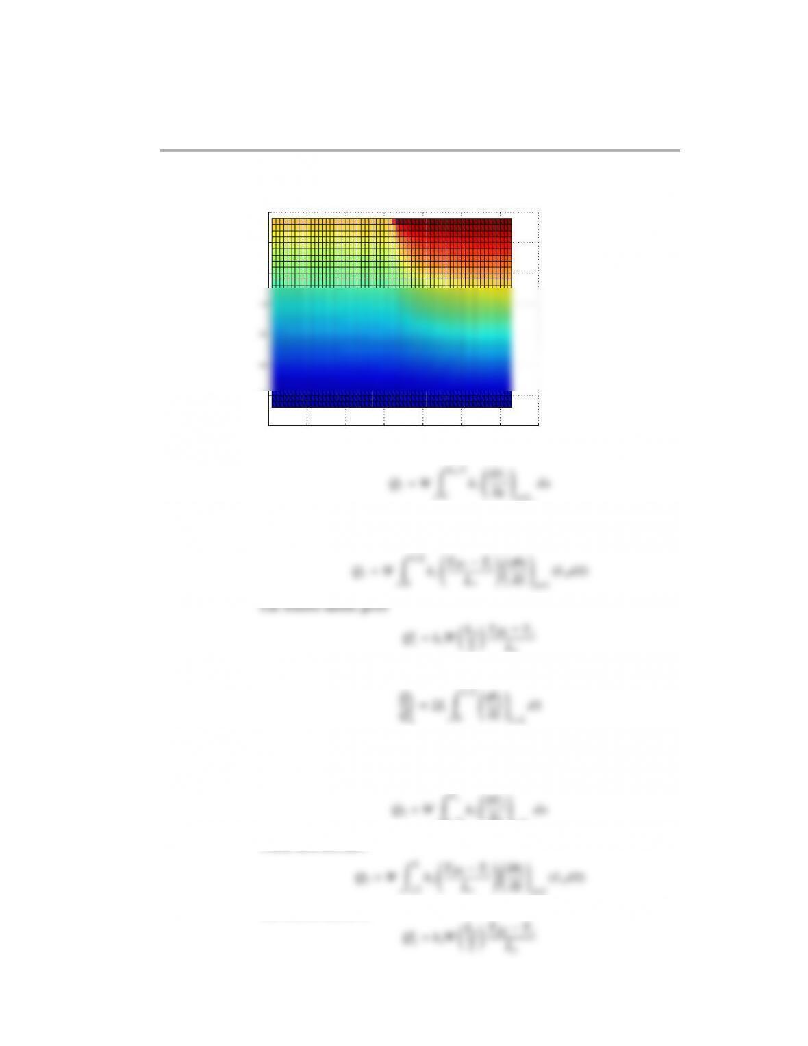
The output of the program is:
462 Partial differential equations
0
5
10
15
20
25
30
35
0 10 20 30 40 50 60 70
S o lu t i on t o s 13 c 1 2p 2
(c) We can write the total flux for material 1 as
0
∂y!y=Ly
where Wis the width of the boundary out of the page . Converting the integral to
dimensionless form gives
The ratio of these two quantities is then
Qr
1
0 dθ1
∂˜y!˜y=L
The integral can be computed directly from the numerical solution since the
problem is solved in dimensionless form.
For material 2, the flux is
Lx/2
∂y!y=Ly
which then becomes
1/2
Lx! ∂θ2
∂˜y!˜y=L