Partial differential equations 423
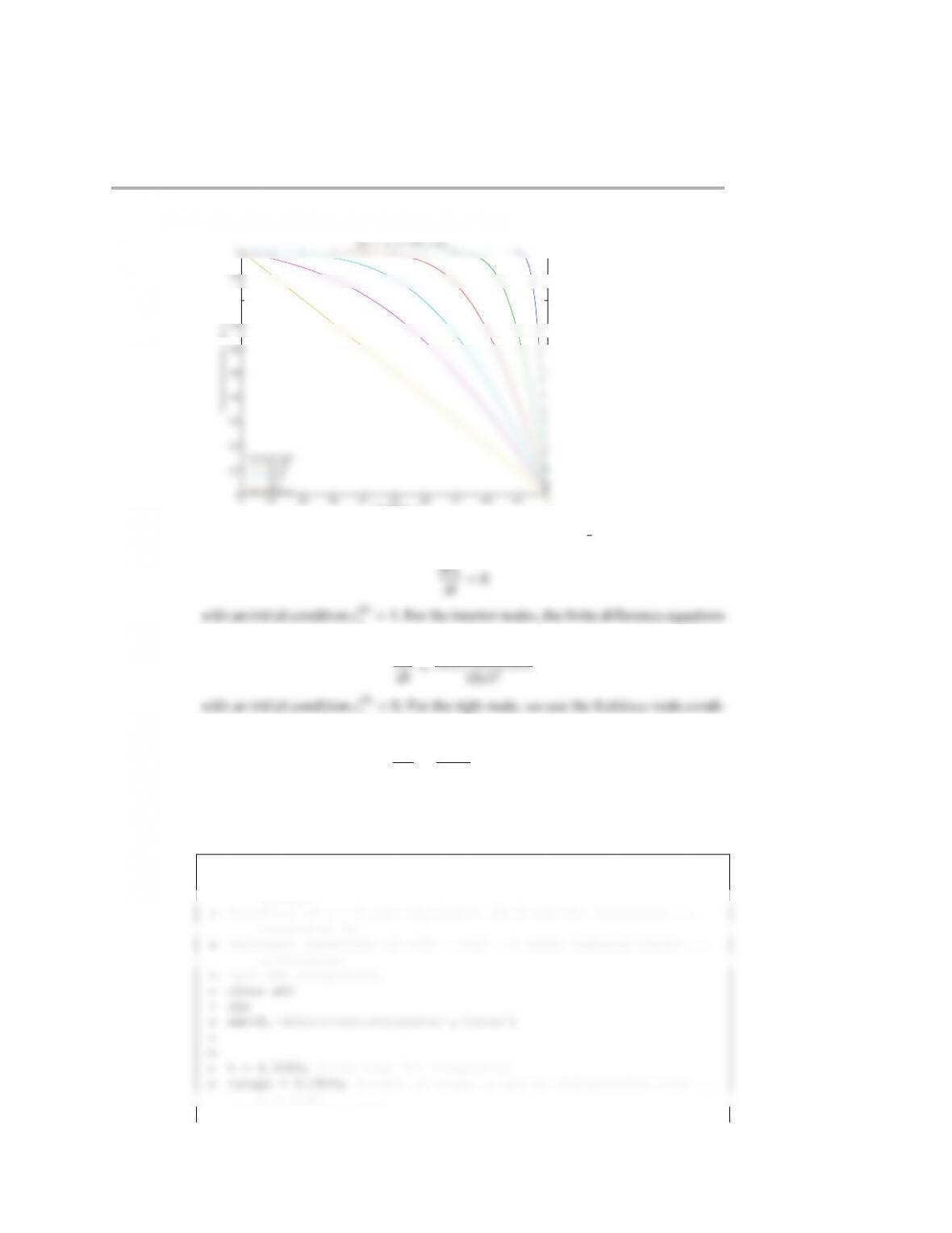
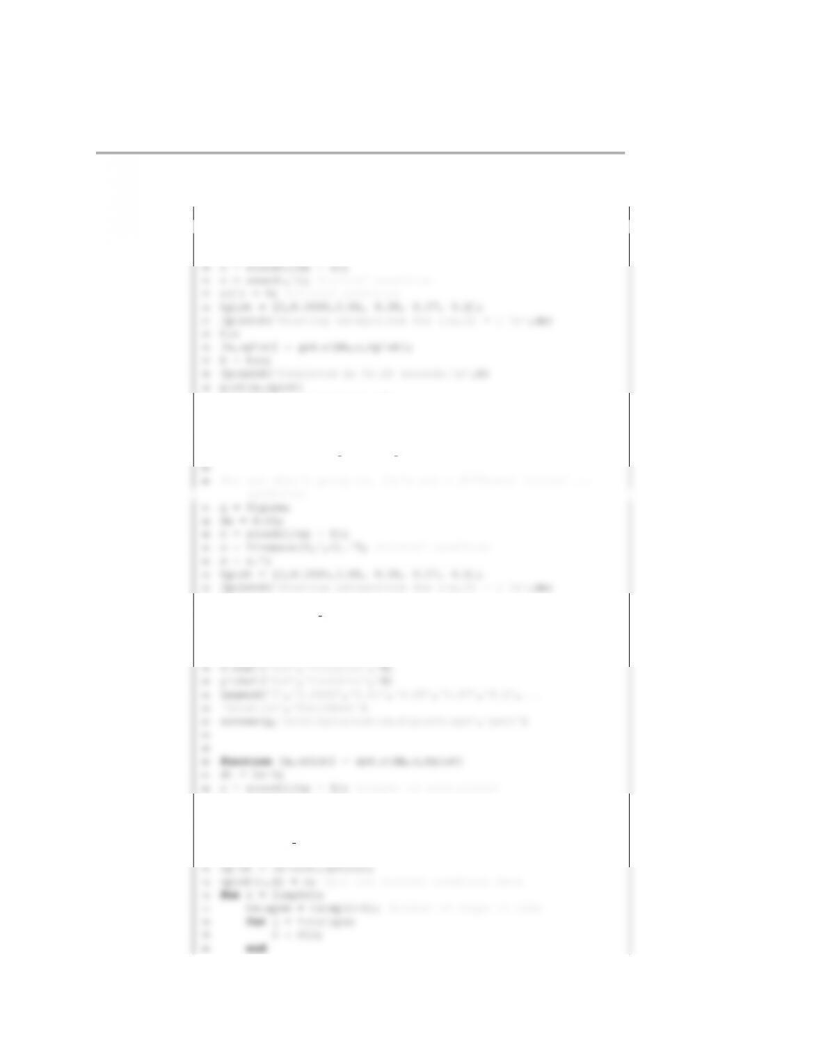
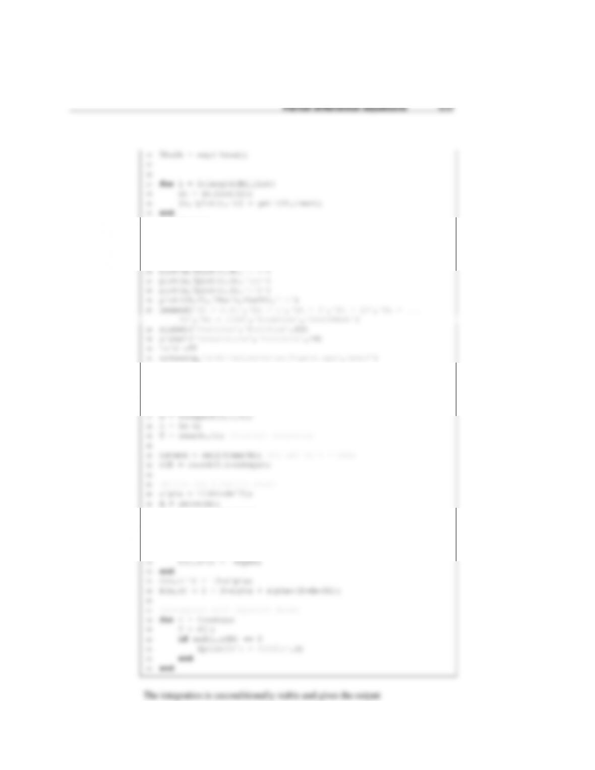
0 0.1 0.2 0.3 0.4 0.5 0.6 0.7 0.8 0.9 1
0
0.1
0.2
0.3
0.4
0.5
0.6
0.7
0.8
0.9
1
P os i ti on , x
C on c e nt r at i on , c(x , t )
S ol u ti o n t o s 13 c 11p 3
0. 0005
0. 005
0. 02
0. 05
0. 1
0. 5
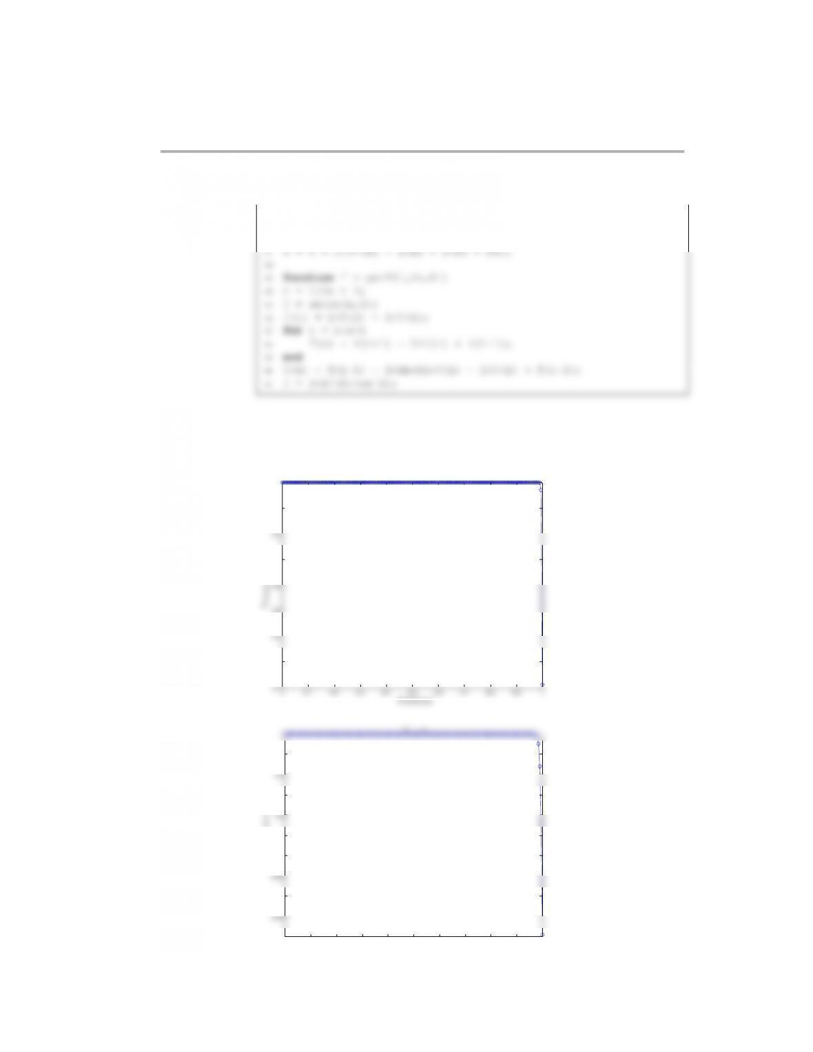
(7.16) The files for this problem are contained in the folder s10c8p1 matlab.
The ODE for the left node is
1=1. For the interior nodes, the finite difference equations
give
dci
=ci+1−2ci+ci−1
i=0. For the right node, we use the fictitious node condi-
tion to get cn+1=cn−1. The ODE is then
dcn
dt
=2
(∆x)2(ci−1−ci)
Note that the kvalue is always zero for node 1.
The Matlab script is:
1function s10c8p1
2%This function solves the unsteady diffusion equation with an …
13 plotsteps = tsteps/10; %frequency for plotting
424 Partial differential equations
14 n = 51; %number of nodes
15 dx = 1/(n-1); %spacing on interval from 0 to 1
26 hold on
27
28
29 %in the time integration, the k values of the first node stays
30 %constant at 0 because the concentrations at this point does …
40
41 for t = 1:tsteps
42
43 %construct the various k values for this time step
44 for i = 2:n
55
56 for i = 2:n
57 k4(i) = dc(c+h*k3,i,dx,n);
58 end
59
69 saveas(figureholder,‘s10c8p1 solution figure.eps’,‘psc2’)
70
71
77 out = (c(i+1) – 2*c(i) + c(i-1))/dxˆ2;
78 end
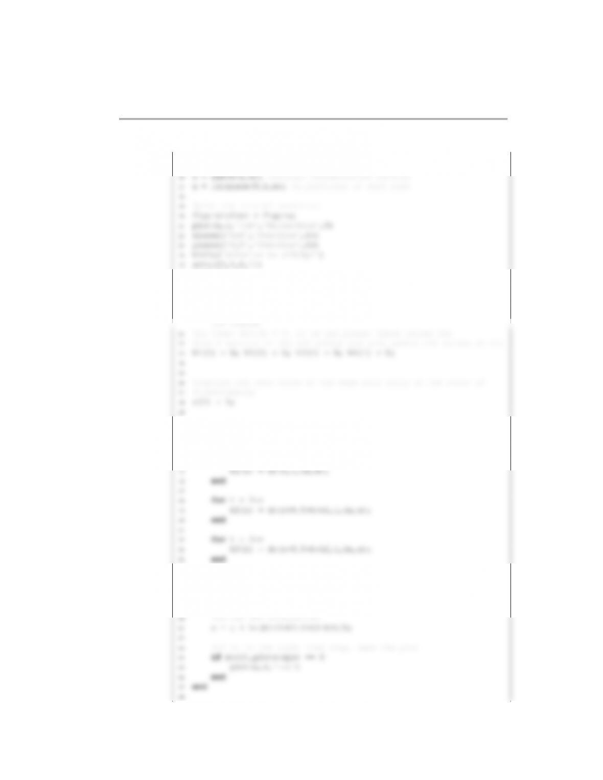
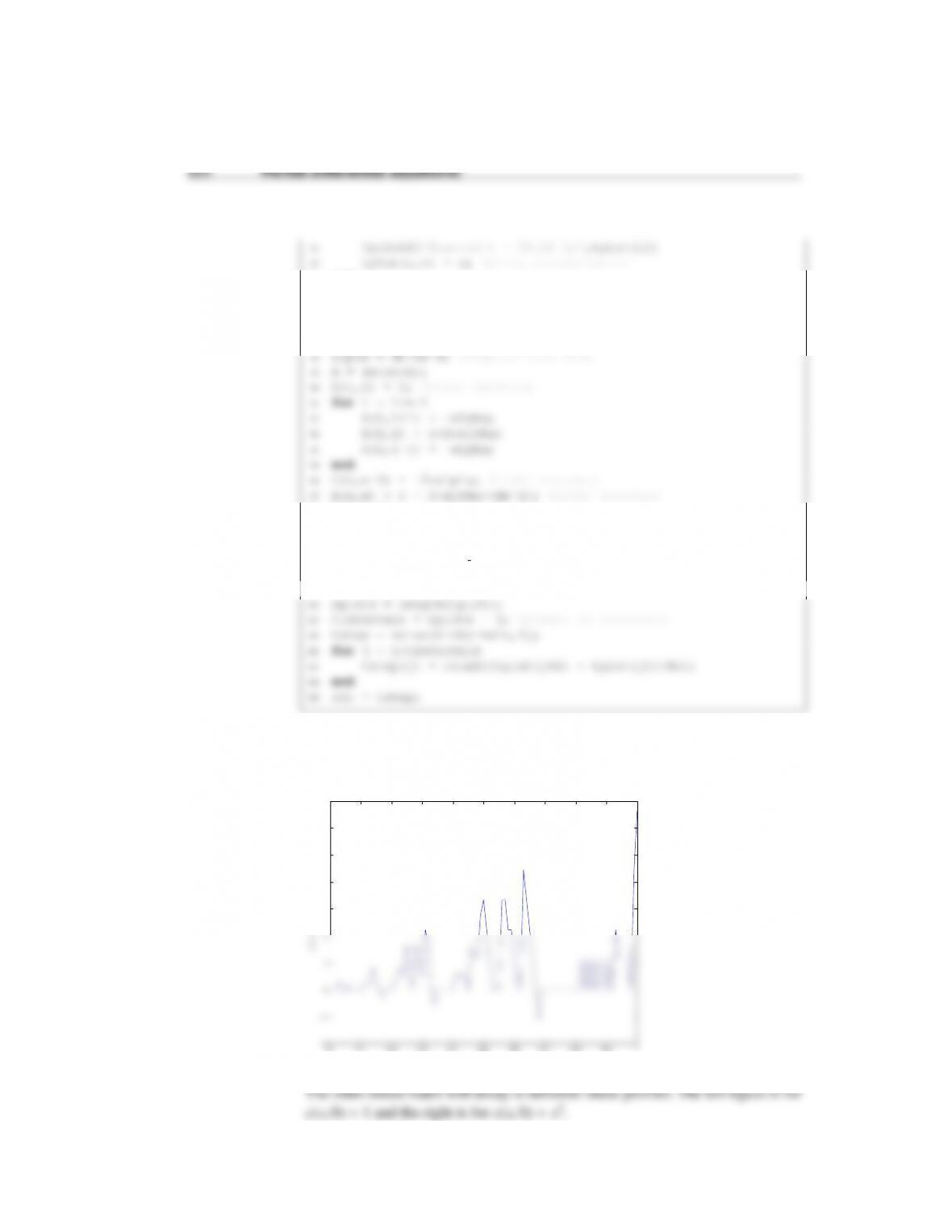
The output file is:
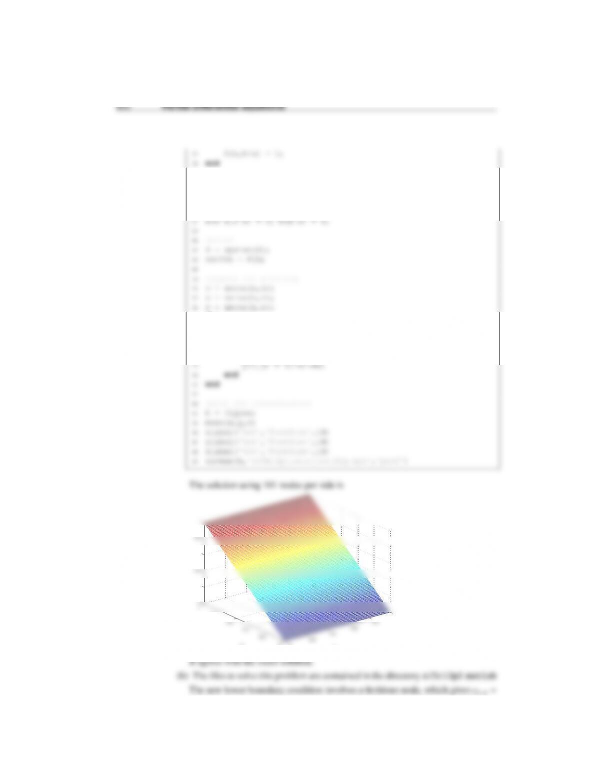
0 0.1 0.2 0.3 0.4 0.5 0.6 0.7 0.8 0.9 1
0
0.1
0.2
0.3
0.4
0.5
0.6
0.7
0.8
0.9
1
x
y
S o lu t io n to s 10 c 8 p 1
(7.17) (a) For the interior nodes, we get
dci
dt
=ci+1−2ci+ci−1
∆x2
For the left node we have
426 Partial differential equations
For the initial condition c(x,0) =x, the initial conditions are
For the initial condition c(x,0=x2, the initial conditions are
(b) For the interior nodes we have
c(k+1)
i−c(k)
i
=c(k+1)
i+1−2c(k+1)
i+c(k+1)
i−1
(c) The files for this problem are contained in the directory s15c11p3 matlab
The Matlab script for this problem is:
1function s15h11p3
2clc
3close all
13 c = linspace(0,1,n).’; %initial condition, transpose to …
right dimension
14 tplot = [0,1e-2]; %points to plot
15 fprintf(‘Starting integration for c(x,0) = x \n’,dx)
16 tic
Partial differential equations 427
27 %to see what’s going on, let’s use a different initial …
condition
28 g = figure;
29 dx = 0.01;
40 xlabel(‘$x$’,‘FontSize’,14)
41 ylabel(‘$c$’,‘FontSize’,14)
42 legend(‘0’,‘0.0005’,‘0.01’,‘0.05’,‘0.07’,‘0.2’,…
43 ‘Location’,‘SouthEast’)
44 saveas(g,‘s15h11p3 solution figure2.eps’,‘psc2’)
54 tic
55 [x,cplot] = get c(dx,c,tplot);
56 t = toc;
57 fprintf(‘Completed in %4.2f seconds.\n’,t)
58 plot(x,cplot)
69 x = linspace(0,1,n); %grid for x positions
70 A = writeA(dt,dx,n); %write the matrix A for future use
71 A = sparse(A); %use sparse solver
72 tstep = get tsteps(tplot,dt);
73 nplots = length(tplot);
83 end
84
85
86 function out = writeA(dt,dx,n)
87 %write the matrix for linear algebra solution
98 out = A;
99
100
101 function out = get tsteps(tplot,dt)
102 %figure out how much to integrate to get to a desired set …
of times
If we give a steady-state initial condition, the result is very stable:
0 0.1 0.2 0.3 0.4 0.5 0.6 0.7 0.8 0.9 1
−2
−1
0
1
2
3
4
5
6
7
x 10−16
x
c(x, 0.01) −x
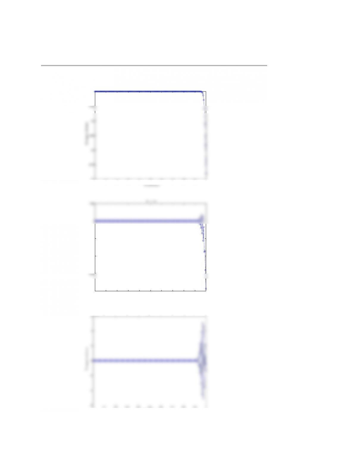
The other initial states will decay to different linear profiles. The left figure is for
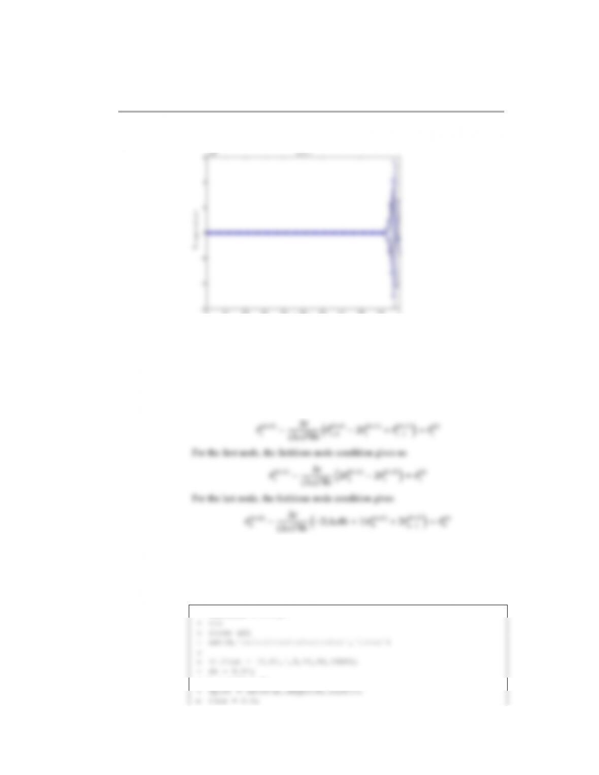
0 0.1 0.2 0.3 0.4 0.5 0.6 0.7 0.8 0.9 1
0
0.5
1
1.5
x
c
0
0 . 0 0 0 5
0 . 0 1
0 . 0 5
0 . 0 7
0 . 2
0 0.1 0.2 0.3 0.4 0.5 0.6 0.7 0.8 0.9 1
0
0.1
0.2
0.3
0.4
0.5
0.6
0.7
0.8
0.9
1
x
c
0
0 . 0 0 0 5
0 . 0 1
0 . 0 5
0 . 0 7
0 . 2
(7.18) The files for this problem are contained in the folder s12c12p12 matlab.
The solution to the PDE from homework #2, problem #3 is
T(x,t)=1
2+
∞
X
4
(2m−1)2π2cos [(2m−1)πx]exp h−(2m−1)2π2ti
duces the ODE
430 Partial differential equations
At the left node, the fictitious node and the boundary condition lead to
In RK4, you need to be very careful with a small value of ∆x. I found a step size
h=10−5to be sufficient to maintain numerical stability but it is slow. Nevertheless,
the numerical solution agrees well with the exact solution.
The Matlab script is:
1function s12c12p12
2clc
3close all
14 T = get T(nx,t,i);
15 err(i,1) = norm(T-baseline);
16 end
17
18
29 ylabel(‘$ | | T{n = 100}– T n | | $’,‘FontSize’,14)
30 legend(‘t = 0.00005’,‘t = 0.001’,‘Location’,‘SouthWest’)
31 saveas(h,‘s12c12p12 solution figure1.eps‘,‘psc2’)
32
33 %number of points for comparison
%6.4f\n’,1/(nx-1))
Partial differential equations 431
37
38 %value of time that we want to use for the comparision
39 t = [0,0.01,0.05,0.1,0.5];
50
51 for j = 1:4
52 %do each piece of integration and then write the end part …
to file
53 tmin = t(j); tmax = t(j+1);
64
65 %compare to baseline value
66 fprintf(‘\n\n\nComparing the time for the solution versus dx\n’)
67 t = 0.01;
68 nmin = 3;
79 errplot(i) = norm(T-baseline);
80 tplot(i) = tcalc;
81 end
82 h = figure;
83 semilogx(errplot,tplot,‘ob’)
93 fprintf(‘\t Starting numerical integration from t = %3.2f to t …
= %3.2f \n’,tmin,tmax)
94 tic
95 nsteps = (tmax-tmin)/h; %number of integration steps to get to …
next t
106 fprintf(‘\t Time required = %8.5f seconds.\n’,tcalc)
107
108
109 function out = feval(T,n)
110 dx = 1/(n-1);
time t with nx
121 %grid points
122 x = linspace(0,1,nx); %make an array of the concentration
123 T = 0.5*ones(1,nx); %this is the first term that is not part …
of the series
Partial differential equations 433
Number of terms in the infinite series, n
100101102
||Tn=100 −Tn||
10-18
10-16
10-14
10-12
10-10
10-8
10-6
10-4
10-2
100
t = 0.00005
t = 0.001
x
0 0.1 0.2 0.3 0.4 0.5 0.6 0.7 0.8 0.9 1
T
0
0.1
0.2
0.3
0.4
0.5
0.6
0.7
0.8
0.9
1
0
0.01
0.05
0.1
0.5
Time for the calculation (seconds)
0.1
0.15
0.2
0.25
(7.19) The files for this problem are contained in the folder s14c11p23 matlab.
(a) For the interior nodes, the ODE we need to solve is
dθi
dτ
= θi+1−2θi+θi−1
Bi(∆x)2!
−
2∆x
=Biθn
so the ODE is
dθn
dτ
= −2(∆xBi +1)θn+2θn−1
Bi(∆x)2!
The program to integrate this with RK4 is
1function s14c11p2
2clc
3close all
9
10 Bi = 1000;
11 [x,T] = getT(Bi,dx,tmax);
12 h = figure;
13 plot(x,T,‘-ob’)
24 ylabel(‘Temperature’,‘FontSize’,14)
25 title(‘Bi = 50’)
26 saveas(h,‘s14c11p2 solution figure2.eps’,‘psc2’)
27
Partial differential equations 435
38 [x,T] = getT(Bi,dx,tmax);
39 h = figure;
40 plot(x,T,‘-ob’)
41 xlabel(‘Position’,‘FontSize’,14)
42 ylabel(‘Temperature’,‘FontSize’,14)
53 saveas(h,‘s14c11p2 solution figure5.eps’,‘psc2’)
54
55 Bi = 1;
56 [x,T] = getT(Bi,dx,tmax);
57 h = figure;
68 h = 1e-4; %make sure still stable
69 T = ones(n,1); %initial condition
70 nsteps = tmax/h; %to get to t = tmax
71 nID = round(0.01*nsteps);
72
83 k1 = getf(T,dx,Bi);
436 Partial differential equations
84 k2 = getf(T + h*k1/2,dx,Bi);
85 k3 = getf(T + h*k2/2,dx,Bi);
86 k4 = getf(T + h*k3,dx,Bi);
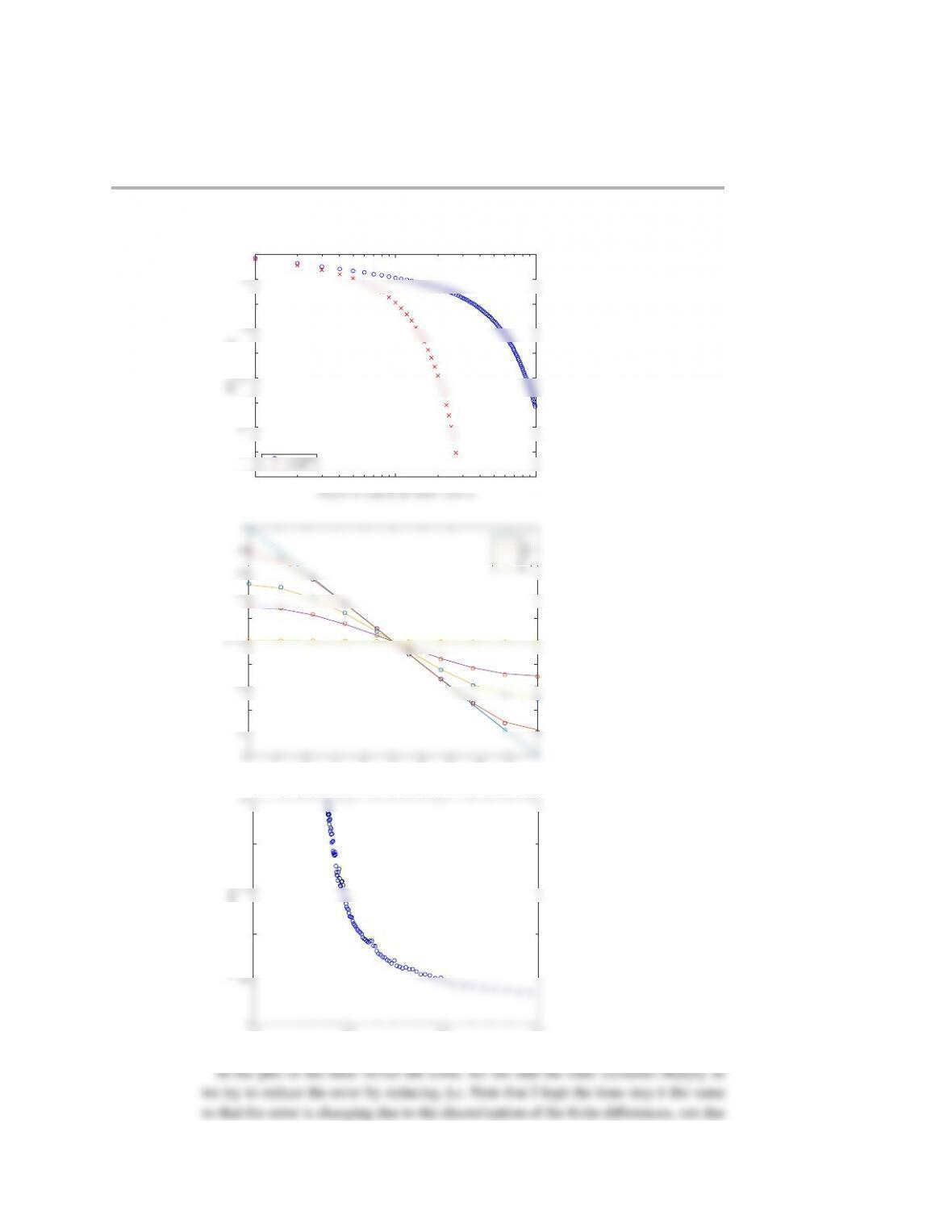
The output for different Bi, in decreasing order, are
0 0.1 0.2 0.3 0.4 0.5 0.6 0.7 0.8 0.9 1
0.2
0.3
0.4
0.5
0.6
0.7
0.8
0.9
1
Pos ition
Te mp erat ure
B i = 1000
0 0.1 0.2 0.3 0.4 0.5 0.6 0.7 0.8 0.9 1
0.5
0.55
0.6
0.65
0.7
0.75
0.8
0.85
0.9
0.95
1
Pos ition
Te mp erature
B i = 5 0
Partial differential equations 437
0 0.1 0.2 0.3 0.4 0.5 0.6 0.7 0.8 0.9 1
0.7
0.75
0.8
0.85
0.9
0.95
1
Pos ition
Te mp erature
B i = 2 0
0 0.1 0.2 0.3 0.4 0.5 0.6 0.7 0.8 0.9 1
0.8
0.85
0.9
0.95
1
1.05
Pos ition
Te mp erature
B i = 1 0
0 0.1 0.2 0.3 0.4 0.5 0.6 0.7 0.8 0.9 1
−6
−4
−2
0
2
4
6
x 1011
Te mp erat ure
B i = 5
438 Partial differential equations
0 0.1 0.2 0.3 0.4 0.5 0.6 0.7 0.8 0.9 1
−6
−4
−2
0
2
4
6
x 1040
Pos ition
Te mp erat ure
B i = 1
What you see here is the onset of the instability of the integration as Bi decreases,
which is equivalent to increasing the dimensionless diffusion coefficient with our
choice of time scale. The instability starts where the concentration is decaying
and eventually propagates to the parts of the solution where we should have a
flat temperature profile for such short times.
(b) The ODEs are linear, so we can rewrite them in a simple form for implicit Euler.
For the interior nodes, we need to solve
∆t
(∆x)2Bi −2(∆xBi +1)θ(k+1)
Notice that the coefficients for the left-hand sides of these equations never change,
while the forcing function on the right-hand side is just the temperature from the
previous step. So this can be efficiently coded by only writing the left-hand side
once at the beginning of the integration:
1function s14c11p3
8n = 1/dx + 1;
18 g = figure;
19 hold on
20 plot(x,Tplot(:,1),‘:ob’)
21 plot(x,Tplot(:,2),‘:xr’)
22 plot(x,Tplot(:,3),‘:*g’)
32
33
34 function [x,T] = getT(Bi,tmax)
35 dx = 0.01;
36 n = 1/dx + 1;
47 A(1,1) = 1 + 2*alpha;
48 A(1,2) = -2*alpha;
49 for i = 2:n-1
50 A(i,i-1) = -alpha;
51 A(i,i) = 1 + 2*alpha;
0 0.1 0.2 0.3 0.4 0.5 0.6 0.7 0.8 0.9 1
0
0.1
0.2
0.3
0.4
0.5
0.6
0.7
0.8
0.9
1
Pos ition
Te mp erat ure
B i = 0. 0 1
B i = 1
B i = 5
B i = 10
B i = 50
B i = 1000
This is what you would have expected from the heat transfer class. For very small
Bi, the thermal conductivity is fast relative to the heat transfer, so the lumped pa-
rameter analysis works. As you increase Bi, the thermal conduction becomes
rather than changing the heat transfer coefficient or the properties of the slab.
(7.20) (a) The files to solve this problem are contained in the directory s15c12p1 matlab
For the interior nodes, the equations are
where kis the node location. For the lower boundary at y=0
ck=0
For the upper boundary at y=1
Partial differential equations 441
1function s15h12p1
2clc
3close all
4set(0,‘defaulttextinterpreter’,‘latex’)
15 k = (i-1)*n + j;
16 A(k,k-n) = 1;
17 A(k,k-1) = 1;
18 A(k,k) = -4;
19 A(k,k+1) = 1;
30 end
31
32 %top nodes
33 i = n;
34 for j = 2:n-1
45 A(k,k) = -4;
46 A(k,k+1) = 2;
47 A(k,k+n) = 1;
48 end
49
59
60 %corners
61 A(1,1) = 1; b(1) = 0;
62 A(n,n) = 1; b(n) = 0;
63 A((n-1)*n+1,(n-1)*n+1) = 1; b((n-1)*n+1) = 1;
74 for i = 1:n
75 for j = 1:n
76 k = (i-1)*n + j;
77 c(i,j) = xsolve(k);
78 x(i,j) = (j-1)*dx;
0
0.2
0.4
0.6
0.8
1
0
0.2
0.4
0.6
0.8
1
0
0.2
0.4
0.6
0.8
1
x
y
c