372 Boundary value problems
57 A(1,1) = 1; b(1) = 1;
58
59 %right BC
60 A(n,n) = 1; b(n) = 0;
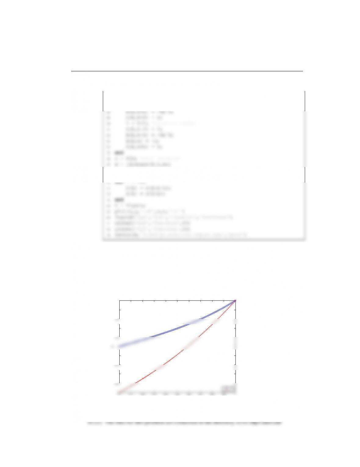
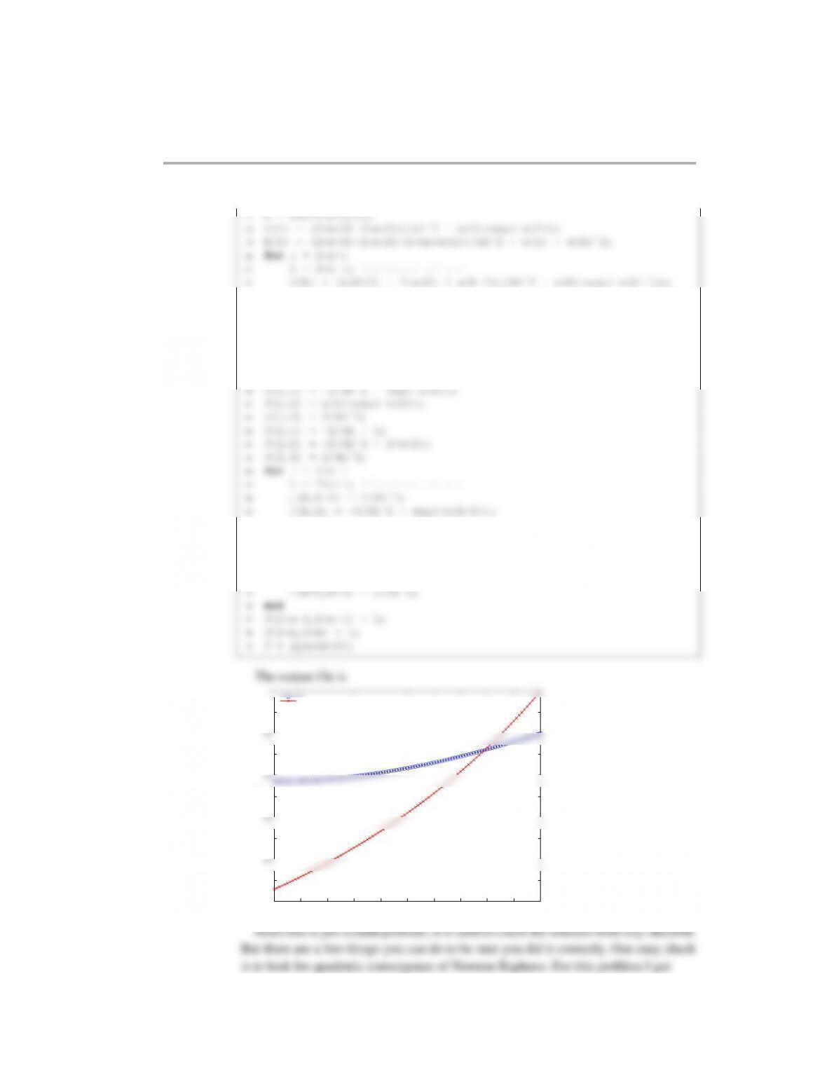
centered finite differences.
(b) The files for this problem are contained in the directory s15c10p2 matlab.
Boundary value problems 373
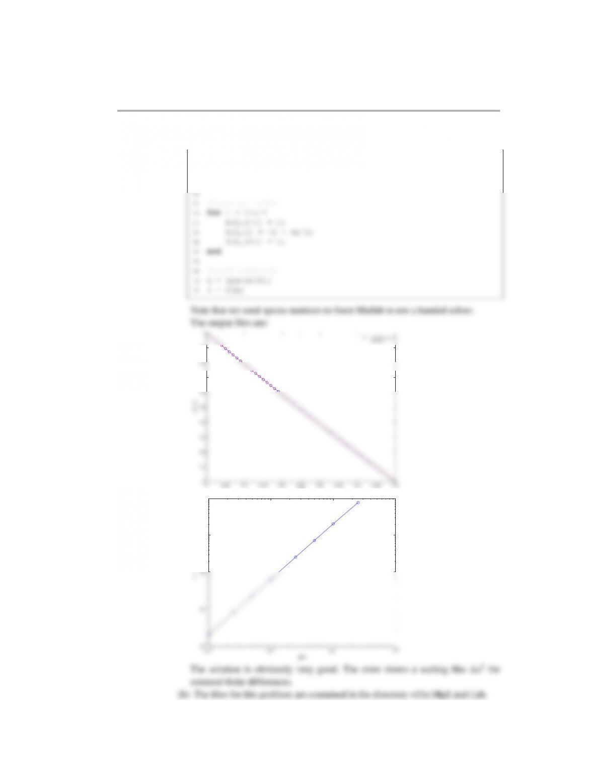
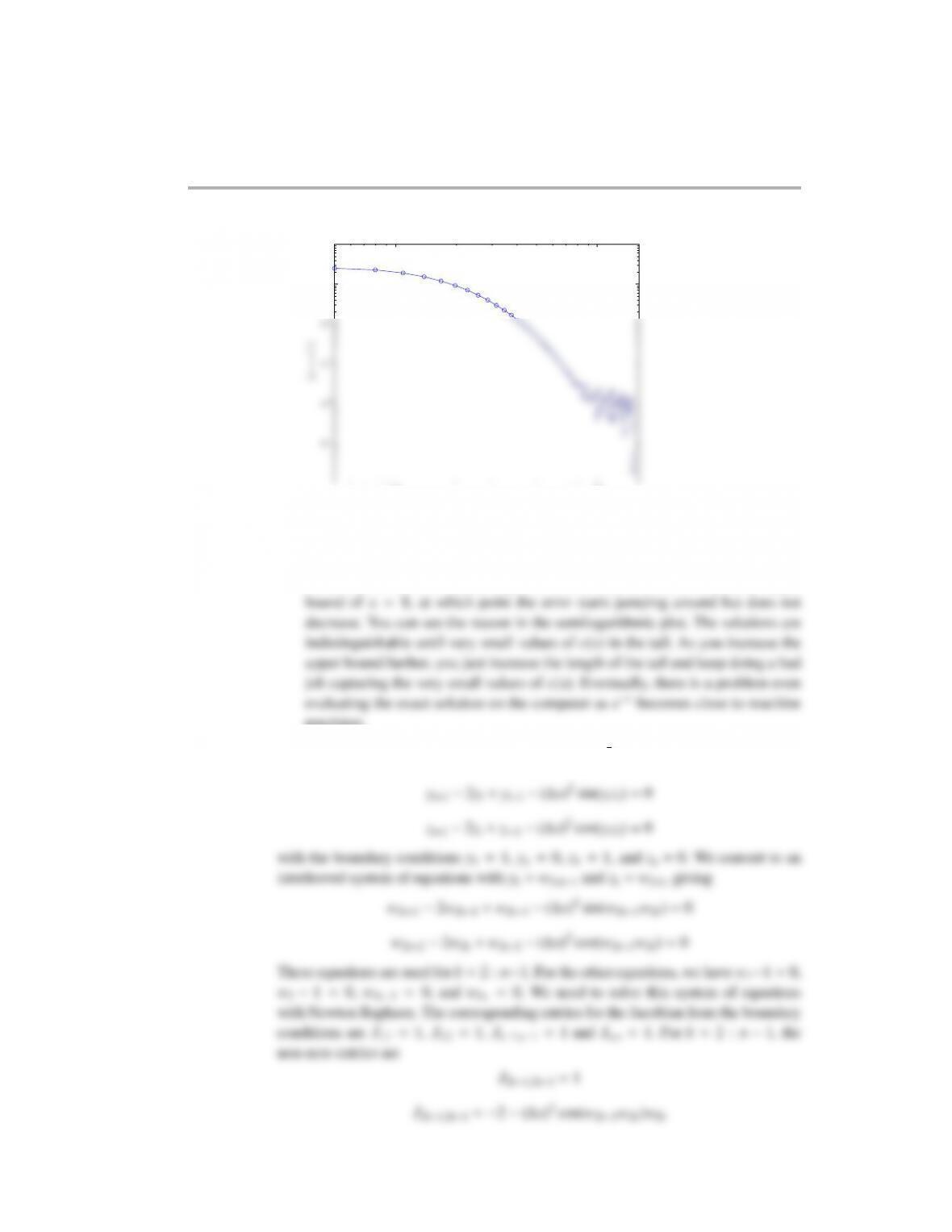
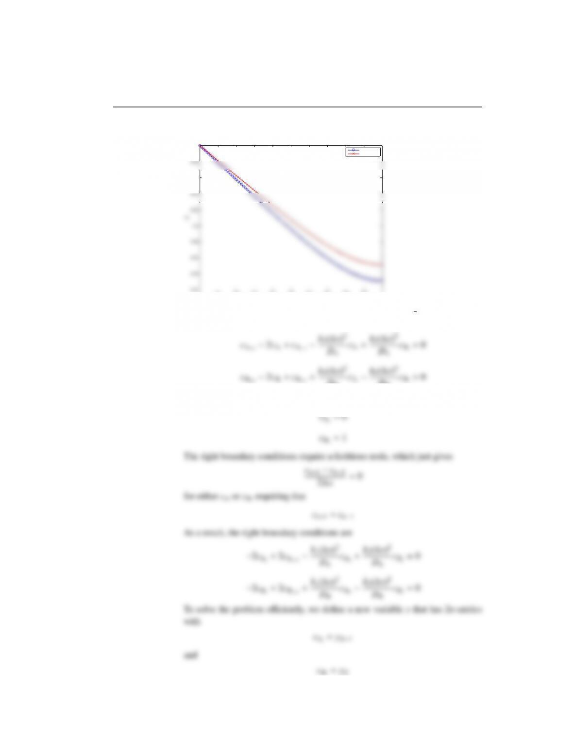
The exact solution now is easiest to write in the form
c=c1e−x+c2ex
The left boundary condition gives c1=1 while the boundary condition at infinity
gives c2=0.
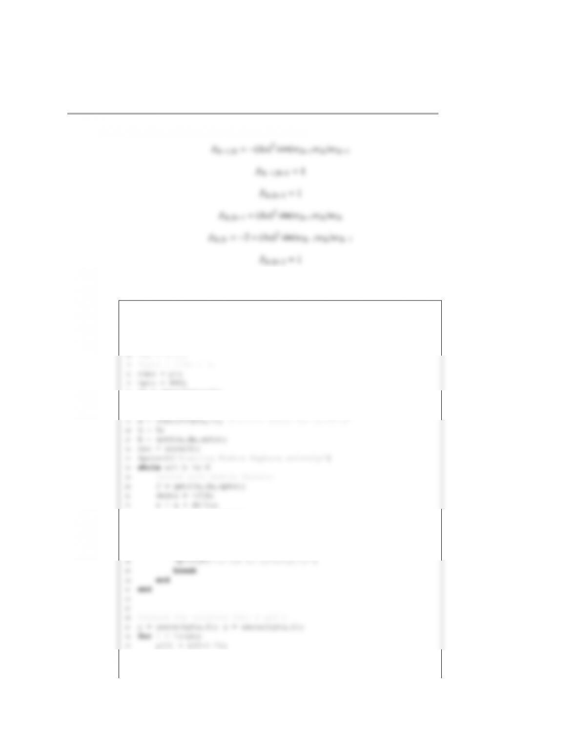
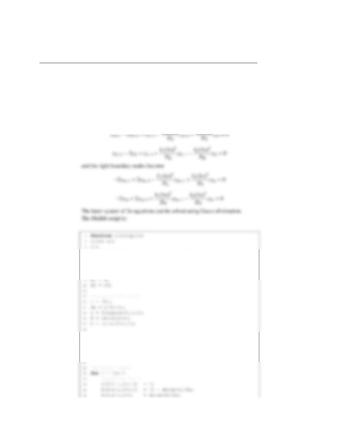
The Matlab program for this problem is
1function s15h10p2
10 Lmax = 15;
11 [xLow,cLow] = solveBVP(dx,xmin,Lmin);
12 [xHigh,cHigh] = solveBVP(dx,xmin,Lmax);
13
14 %exact solution
25 saveas(h,‘s15h10p2 solution fig1.eps’,‘psc2’)
26
27 h = figure;
28 plot(xHigh,cHigh,‘ob’,xHigh,c exactHigh,‘-r’)
29 xlabel(‘$x$’,‘FontSize’,14)
40 legend boxoff
41 saveas(h,‘s15h10p2 solution fig3.eps’,‘psc2’)
42
43 %compute the error as a function of dx
44 nplot = 50;
374 Boundary value problems
48 xmax = L plot(i);
49 [x,c] = solveBVP(dx,xmin,xmax);
50 c exact = exactSolution(dx,xmin,xmax);
57 ylabel(‘$ | | c – c ˆ *||$’,‘FontSize’,14)
58 saveas(h,‘s15h10p2 solution fig4.eps’,‘psc2’)
69 n = round((xmax-xmin)/dx) + 1; %make an integer
70 x = linspace(xmin,xmax,n);
71
72 A = zeros(n,n);
73 b = zeros(n,1);
84 A(i,i) = -2 – dxˆ2;
85 A(i,i+1) = 1;
The output files are
Boundary value problems 375
0 0.05 0.1 0.15 0.2 0.25 0.3 0.35 0.4 0.45 0.5
0
0.1
0.2
0.3
0.4
0.5
0.6
0.7
0.8
0.9
1
x
c(x)
N u m e r ic a l
E x ac t
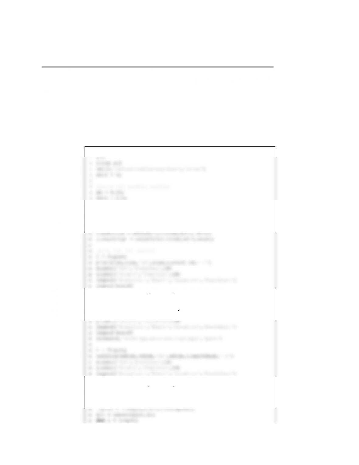
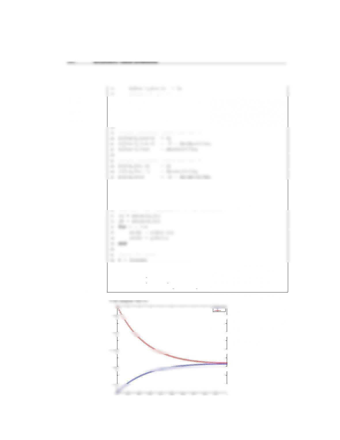
0 5 10 15
0
0.1
0.2
0.3
0.4
0.5
0.6
0.7
0.8
0.9
1
x
c(x)
N u m e r ic a l
E x ac t
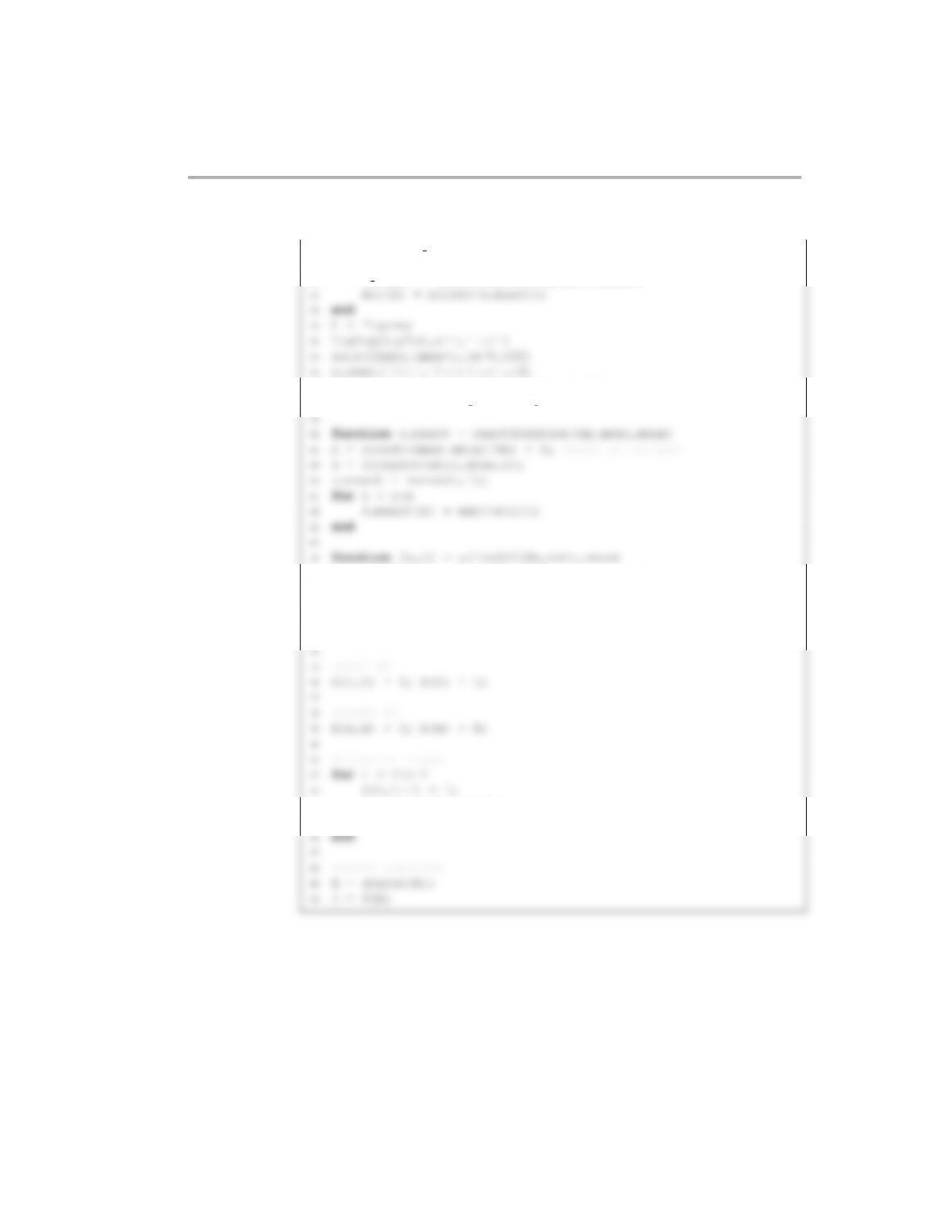
10−7
10−5
10−4
10−3
10−2
10−1
100
x
N u m e r ic a l
E x ac t
376 Boundary value problems
100101
10−4
10−3
10−2
10−1
100
101
L
||c−c∗||
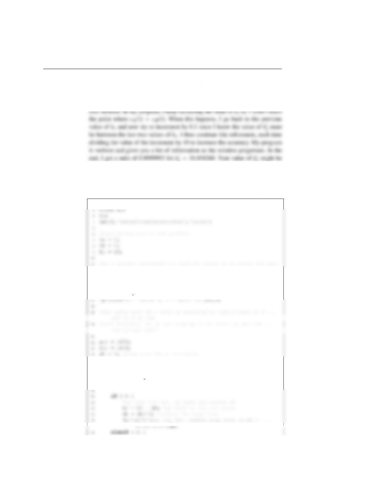
As you might expect, using x=0.5 as the upper bound is way too close to
the start of the problem and the numerical solution is far from the exact result.
However, when we put the boundary far away, the solution is quite good. In
the error, we see a continual improvement in the error out to around an upper
precision.
(6.20) The files for this problem are in the folder s13c11p2 matlab.
When you convert to finite differences, you get the equations
Boundary value problems 377
The Matlab script for this problem is:
1function s13c11p2
2clc
3close all
4set(0,‘defaulttextinterpreter’,‘latex’)
5
10 dx = xmax/(npts-1);
11 x = linspace(0,xmax,npts);
12
23 R = getR(w,dx,npts);
24 k=k+1;
25 err = norm(R);
26 fprintf(‘k = %2d \t err = %6.4e \n’,k,err)
27 if k>20
38 z(i) = w(2*i);
39 end
40
378 Boundary value problems
41 h = figure;
52 R = zeros(npts,1);
53 R(1,1) = w(1)-1; %left BC on y
54 R(2,1) = w(2)-1; %left BC on z
55 for k = 2:npts-1
56 %write the interior node equations
65 J(1,1) = 1;
66 J(2,2) = 1;
67 for k = 2:npts-1
68 %derivatives of the BVP for y
69 r=2*k-1;
80 J(r,2*k-1) = dxˆ2*sin(w(2*k-1)*w(2*k))*w(2*k);
81 J(r,2*k) = -2 + dxˆ2*sin(w(2*k-1)*w(2*k))*w(2*k-1);
82 J(r,2*k+1) = 0;
83 J(r,2*k+2) = 1;
84 end
Boundary value problems 379
0 0.5 1 1.5 2 2.5 3 3.5
−0.8
−0.6
−0.4
−0.2
0
0.2
0.4
0.6
0.8
1
x
yor z
S ol ut io n t o s 13c 11 p2
y
z
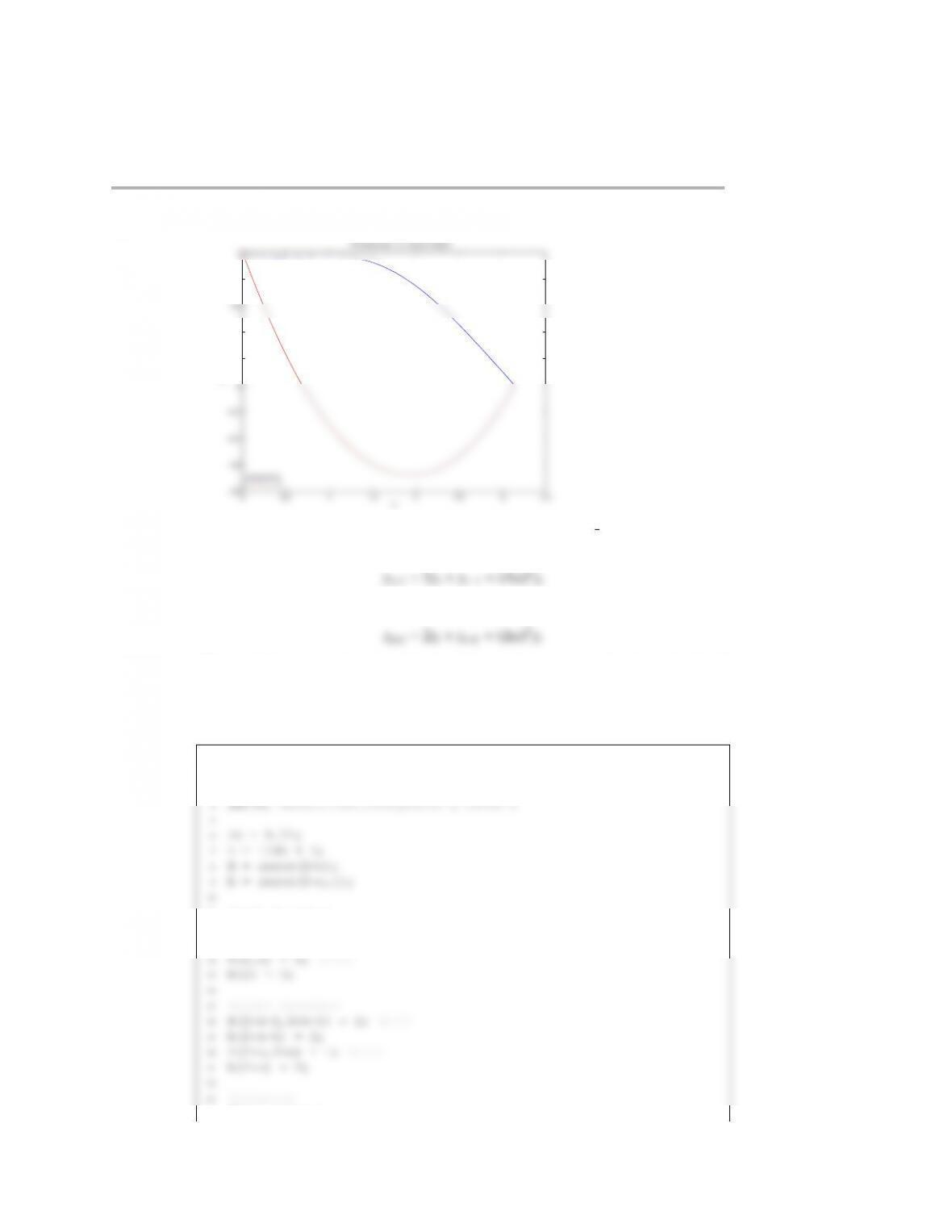
(6.21) The files for this problem are contained in the folder s14c11p1 matlab.
The finite difference equations are
and
The variables are interleaved in the program as [y1,z1,y2,z2, . . .] to keep the band
structure. The problem itself is linear, so we just solve it with a linear solver.
The Matlab program is
1function s14c11p1
2clc
3close all
11 %left boundary
12 A(1,1) = 1; %y(0)
13 b(1) = 1;
380 Boundary value problems
25 k=2*i-1; %equation number
26 A(k,k-2) = 1;
27 A(k,k) = -2;
38 y = zeros(n,1);
39 z = zeros(n,1);
and the output is
0 0.1 0.2 0.3 0.4 0.5 0.6 0.7 0.8 0.9 1
0
0.2
0.4
0.6
0.8
1
1.2
1.4
1.6
1.8
2
x
y
z
Boundary value problems 381
We can arrange the solution into a 2n×1 vector
x1
y1
x2
y2
yn
For the interior node equations, we have
∆z2−xi−y2
For conversion to entries in w, I like to define k=2i−1 as the location of xito make
the code look a bit cleaner.
For the right boundary nodes, we have easy equations
and
For the left boundary nodes, we need fictitious nodes x0and y0. For the xboundary
condition, we have
2∆z
which gives x2=x0and thus
∆z2−x1e−y1=0
For the right boundary node, we have
∆z2−x1−y2
382 Boundary value problems
Writing everything in the form of a residual and the variable wgives
.
.
.
w2n−1−0.8
w2n−1
where k=2i−1 for i=2 : n−1.
The entries in the first row of the Jacobian are
J1,1=−2
∆z2
For the interior nodes with k=2i−1 we have
Jk,k−2=1
∆z2
Jk,k=−2
Boundary value problems 383
For the right boundaries the Jacobian entries are
J2n−1,2n−1=1
and
The Matlab program that solves this problem is
11 %setup problem
12 w = zeros(2*n,1); %initial guess
13 R = getR(w,n,dz);
14 k = 1;
15 tol = 1e-8;
26 break
27 end
28 end
29
30 %unpack results
41 legend(‘$x$’,‘$y$’,‘Location’,‘NorthWest’)
42 legend boxoff
43 saveas(h,‘s15h10p3 solution fig.eps’,‘psc2’)
44
45
384 Boundary value problems
53 R(k+1) = (w(k+3) – 2*w(k+1) + w(k-1))/dzˆ2 – w(k) – w(k+1)ˆ2;
54 end
55 R(2*n-1) = w(2*n-1) – 0.8;
56 R(2*n) = w(2*n) – 1;
57
58 function J = getJ(w,n,dz)
59 J = zeros(2*n);
70 J(k,k+1) = w(k)*exp(-w(k+1));
71 J(k,k+2) = 1/dzˆ2;
72 J(k+1,k-1) = 1/dzˆ2;
73 J(k+1,k) = -1;
74 J(k+1,k+1) = -2/dzˆ2 – 2*w(k+1);
0 0.1 0.2 0.3 0.4 0.5 0.6 0.7 0.8 0.9 1
0
0.1
0.2
0.3
0.4
0.5
0.6
0.7
0.8
0.9
1
z
x,y
x
y
Boundary value problems 385
1k = 1 norm(R) = 1.2806e+00
2k = 2 norm(R) = 5.2442e+00
This was quite useful in debugging, since for a while I was getting a small value of
||R|| without quadratic convergence, which was due to a typo in the Jacobian! You can
also look at the solution and see if the boundary conditions are satisfied. This seems
to be the case.
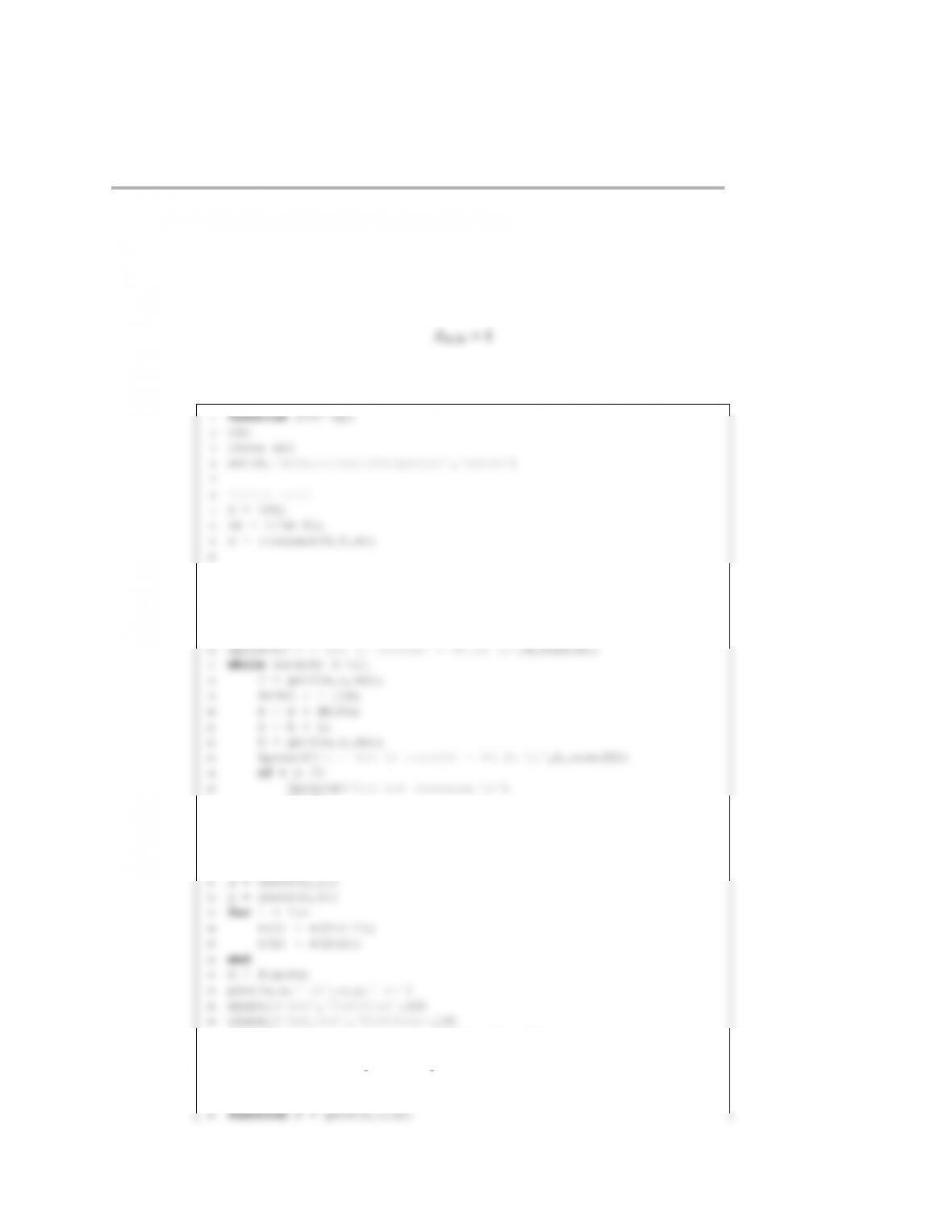
(6.23) The files for this problem are contained in the folder s14c10p23 matlab.
(a) This is a linear problem. The finite difference approximation is
∆x2=x3
which I will code as
At the left boundary, we just have
At the right boundary, the fictitious node condition is
2∆x
which gives us
These are linear equations that are easily solved.
The Matlab program is
1function s14c10p2
2clc
13 b(1) = 1; %left boundary
14 for i = 2:n-1
15 %interior nodes
16 A(i,i-1) = 1;
17 A(i,i) = -2 – dxˆ2*x(i)ˆ3 ;
386 Boundary value problems
20 %right boundary
28 plot(x,y,‘-ob’)
29 ylabel(‘$y$’,‘FontSize’,14)
30 xlabel(‘$x$’,‘FontSize’,14)
31 saveas(h,‘s14c10p2 solution figure.eps’,‘psc2’)
(b) For the nonlinear problem, the interior nodes change to
and the right boundary changes to
The first row of the Jacobian is just J1,1=1. For the interior rows, the non-zero
entries are
The Matlab program is
1function s14c10p3
2clc
13 A(1,1) = 1; %left boundary
14 b(1) = 1; %left boundary
15 for i = 2:n-1
16 %interior nodes
17 A(i,i-1) = 1;
Boundary value problems 387
25
26 %solve the nonlinear problem
27 k = 1;
28 y = y linear; %use as initial guess
39 end
40
41 %plot
42 h = figure;
43 plot(x,y linear,‘-ob’,x,y,‘-xr’)
54 R(i,1) = y(i+1) – 2*y(i) + y(i-1) – dxˆ2*x(i)ˆ3*y(i)ˆ2;
55 end
56 R(n,1) = 2*y(n-1) – 2*y(n) – dxˆ2*x(n)ˆ3*y(n)ˆ2;
57
58 function J = getJ(y,x,dx)
388 Boundary value problems
0 0.1 0.2 0.3 0.4 0.5 0.6 0.7 0.8 0.9 1
0.82
0.84
0.86
0.88
0.9
0.92
0.94
0.96
0.98
1
x
y
L i n e a r
N o n l i n e a r
(6.24) The files for this problem are contained in the folder s12c11p123 matlab.
(a) First convert the equations using the finite difference approximation
DB
DB
The left boundary conditions are simple:
Boundary value problems 389
We then can rewrite the left boundary conditions as
y1=0
y2=0
The interior nodes become
4set(0,‘defaulttextinterpreter’,‘latex’)
5
6%parameters in the problem
7Da = 2;
8Db = 1;
19 %left boundary condition for A
20 A(1,1) = 1; b(1) = 0;
21
22 %left boundary condition for B
23 A(2,2) = 1; b(2) = 1;
33 A(2*i,2*i-2) = 1;
34 A(2*i,2*i-1) = dx*dx*k1/Db;
35 A(2*i,2*i) = -2 – dx*dx*k2/Db;
36 A(2*i,2*i+2) = 1;
37 end
48
49 %solve the ODE
50 A = sparse(A); %makes the solution faster
51 y=A\b;
52
63 plot(x,ca,‘-ob’,x,cb,‘-or’)
64 xlabel(‘$x$’,‘FontSize’,14)
65 ylabel(‘$c i$’,‘FontSize’,14)
66 legend(‘$c a$’,‘$c b$’)
67 saveas(h,‘s12c11p123 solution figure1.eps’,‘psc2’)
0 0.1 0.2 0.3 0.4 0.5 0.6 0.7 0.8 0.9 1
0
0.1
0.2
0.3
0.4
0.5
0.6
0.7
0.8
0.9
1
x
ci
ca
cb
Boundary value problems 391
(b) In my bracketing method, I used the fact that for k2=0 the solution is cA=0
everywhere. So I can gradually increase the value of k2and the value of cA(1) will
2=10.454260. Your value of k∗
2might be
slightly different since I allow you to stop for any value of k2where the ratio is
offin the 7th decimal place.
The Matlab script is:
1function s12c11p123b
12 %concentrations are the same
13
14 %Start with no reverse reaction
15 k2 = 0;
16 r = compute c(Da,Db,k1,k2);
25 fprintf(‘\n****************************************\n’)
26 fprintf(‘Starting bracketing procedure\n’)
27 while err >tol
28 r = compute c(Da,Db,k1,k2); %new value of r
29 fprintf(‘k2 = %8.6f \t r = %8.7f \n’,k2,r)