
6Boundary value problems
354 Boundary value problems
Problems
(6.1)
(6.2)
(6.3) c0=c2
(6.5) From the boundary conditions, we have y1=0 and y3=1. From the number of
nodes, we also have ∆x=1/2. Discretizing the equation for the interior node,
(6.6) The Taylor series expansions for each of these terms are
yi+2=y+y′(2∆x)+1
2y′′(2∆x)2+1
6y′′′(2∆x)3
yi+1=y+y′(∆x)+1
2y′′(∆x)2+1
6y′′′(∆x)3
Boundary value problems 355
(6.7) (a) The Taylor series is
(b) We need 5 points, so j∈[−2,2].
(c) There are 4 equations.
(d) From the Taylor series
we have the equations
If we multiply each equation by wj, we want to remove all the lower derivatives
and leave only the highest derivative. The first derivative is removed by requiring
(6.8) With 5 nodes, we have ∆x=0.25. Using the product rule on the left-hand side,
Using centered finite differences, we get (for interior nodes)
(∆x)2!yi+yi+1−yi−1
2∆x2
356 Boundary value problems
The five residual equations are
The elements of the Jacobian are
(6.9) The left node and the two interior nodes are easy to compute
c1−1=0
c3−2c2+c1=0
0 0 1 (2∆xk/D)c4−1
(6.10) The discretized equations are
w4−2w3+w2
∆z2=x4−x2
2∆z
+w3
x4−2x3+x2
3w3
∆z2=y2
(6.11) If we make a vector ythat interleaves the values of aand bover the 4 nodes, we have
y=
y1
y2
y3
y4
=
a1
b1
a2
b2
(∆x)2+b2
Rewriting in terms of y,
R2=2y4−2y2
(∆x)2+y2
2=0
(∆x)2−y2
358 Boundary value problems
The fourth residual is the interior node for b2at x=1/3
(∆x)2= 1
3!2
which becomes
(∆x)2−4y5
9+y2
The last two nodes require using the boundary conditions. The seventh residual uses
the boundary condition on ausing a fictitious node a5,
a5−a3
2∆x
=2
(6.12) The exact solution is a sum of exponentials
c(x)=c1exp( √Dax)+c2exp(−√Dax)
The finite-difference approximation to the equation is
ci+1−2ci+ci−1
Boundary value problems 359
difference approximation. The error goes to zero as the Damkohler number goes to
(6.13) (a) xn=2
(b) The differential equation is
d2c
dx2=c2
(c) The left boundary condition is c(x=0) =1. The right boundary conditions
dc/dx =cat x=2.
(d) A suitable function would be
Computer Problems
(6.14) The files for this problem are contained in the folder s12c10p3 matlab.
The interior nodes for
d2y
dx2=0
have the normal form for centered finite differences,
2cn−1−2cn−2∆xc3/2
n=0
360 Boundary value problems
This is a nonlinear system that needs to be solved by Newton-Raphson. The non-zero
entries to the Jacobian are:
dy
dx
=a=−(a+1)3/2
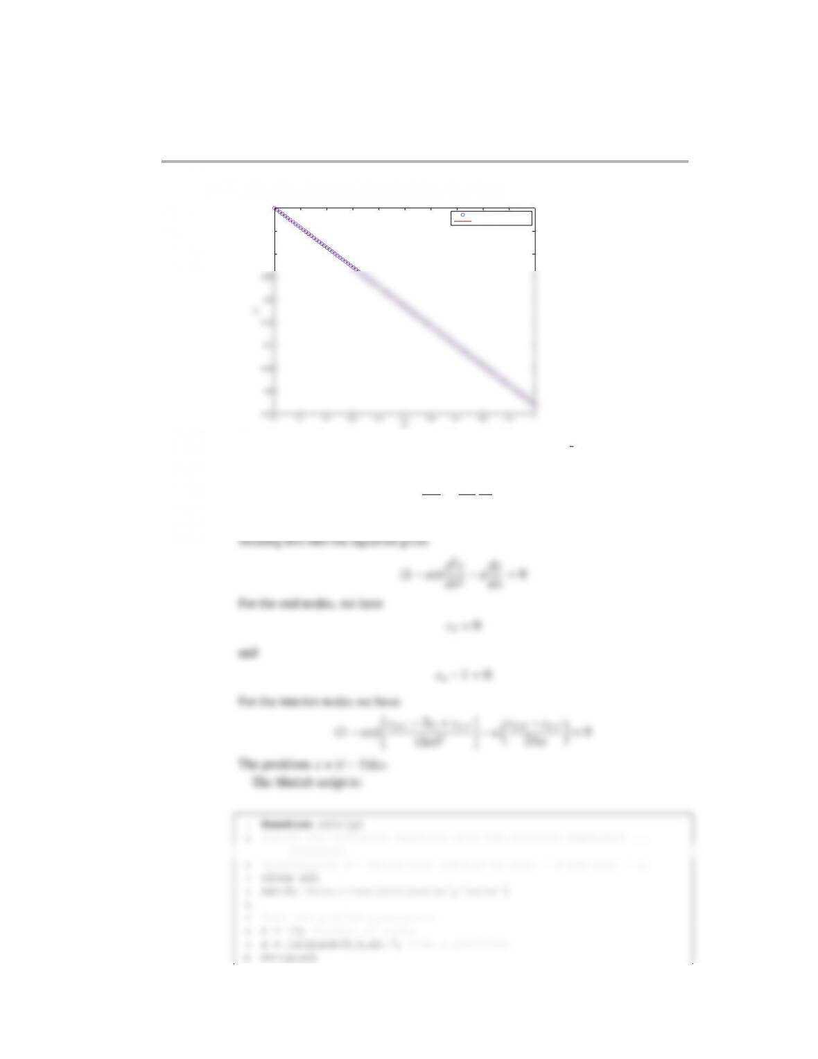
To find the slope, you need to solve the nonlinear equation using Newton’s method
for
f(a)=(a+1)3/2+a
The slope from Newton’s method is a=−0.4302 and the result agrees very nicely
with the solution from finite differences.
10 err = norm(R);
11 count = 0;
12 fprintf(‘Solve the nonlinear ODE\n’)
13 fprintf(‘k = %2d \t err = %8.6e \n’,count,err)
14 while err >10ˆ-8
Boundary value problems 361
21 fprintf(‘k = %2d \t err = %8.6e \n’,count,err)
22 if count >20
23 fprintf(‘Failed to converge.\n’)
24 y = 0;
35 end
36 yexact = c*x+1;
37 fprintf(‘The slope of the exact solution is %6.4f \n’,c)
38
39 h = figure;
50
51 function out = fder(c)
52 out = 1.5*(c+1)ˆ(1/2) + 1;
53
54 function out = residual(y,n)
65 for i = 2:n-1
66 out(i,i-1) = 1;
67 out(i,i) = -2;
68 out(i,i+1) = 1;
69 end
362 Boundary value problems
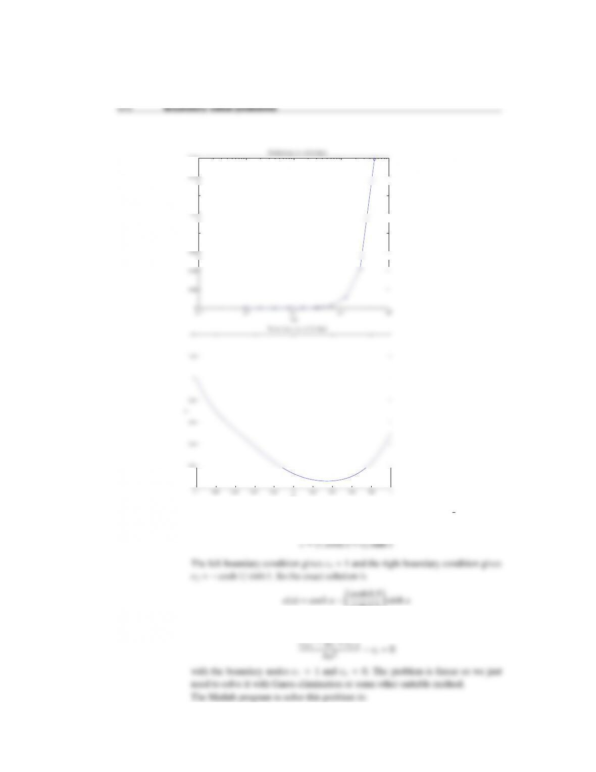
0 0.1 0.2 0.3 0.4 0.5 0.6 0.7 0.8 0.9 1
0.55
0.6
0.65
0.7
0.75
0.8
0.85
0.9
0.95
1
x
y
N u m e r ic al I n t e gr at ion
E x ac t I n te g ra t ion
(6.15) The files for this problem are contained in the folder s10c7p1 matlab.
If we differentiate the terms with the product rule, we get
Dd2c
dx2+dD
dx
dc
dx
=0
The position dependent diffusivity D=D0(1 −ax) acts like a convection term. Sub-
Boundary value problems 363
11 axis([0,1,0,1])
17 case 1
18 plot(x,c,‘-ob’)
21 case 3
22 plot(x,c,‘-*g’)
25 case 5
26 plot(x,c,‘-dm’)
27 end
28 end
29 xlabel(‘$x$’,‘FontSize’,14)
40 A(1,1) = 1; b(1) = 1;
41 A(n,n) = 1; b(n,1) = 0;
42
43 %write the interior nodes
44 for i = 2:n-1
Boundary value problems 365
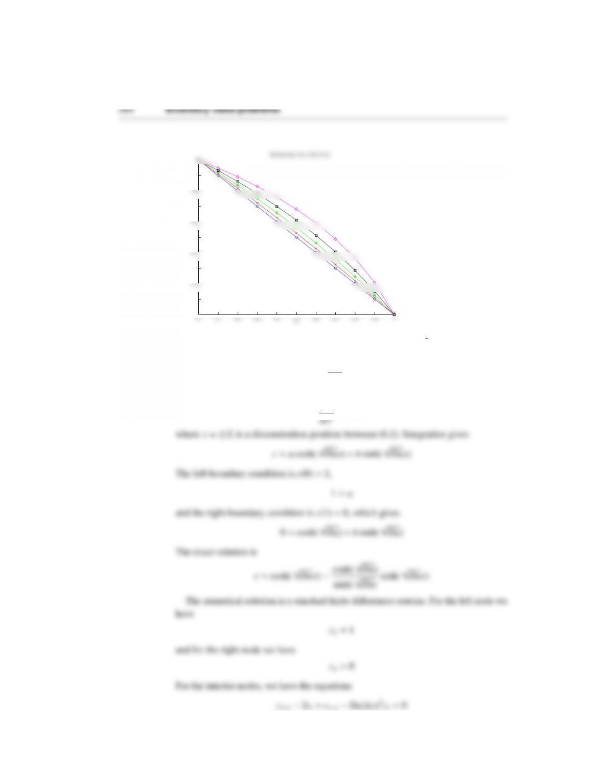
where ∆x=(n−1)−1is the grid spacing. This is just a linear set of equations, so you
can solve it with the slash command.
The Matlab script is:
1function s12c10p1
12 end
13 [cexact(i,:),x] = compute cexact(Da,1000);
14 end
15 h = figure;
16 loglog(nplot,errplot,‘-o’)
26 legend(‘Da = 0.01’,‘Da = 0.1’,‘Da = 1’,‘Da = 10’,‘Da = …
100′,‘Da = 1000’)
27 saveas(h,‘s12c10p1 solution figure2.eps’,‘psc2’)
28
29 function out = get err(n,Da)
40 A(i,i) = -2 – Da*dx*dx;
41 A(i,i+1) = 1;
42 %the constant is zero
43 end
44 %right boundary condition
366 Boundary value problems
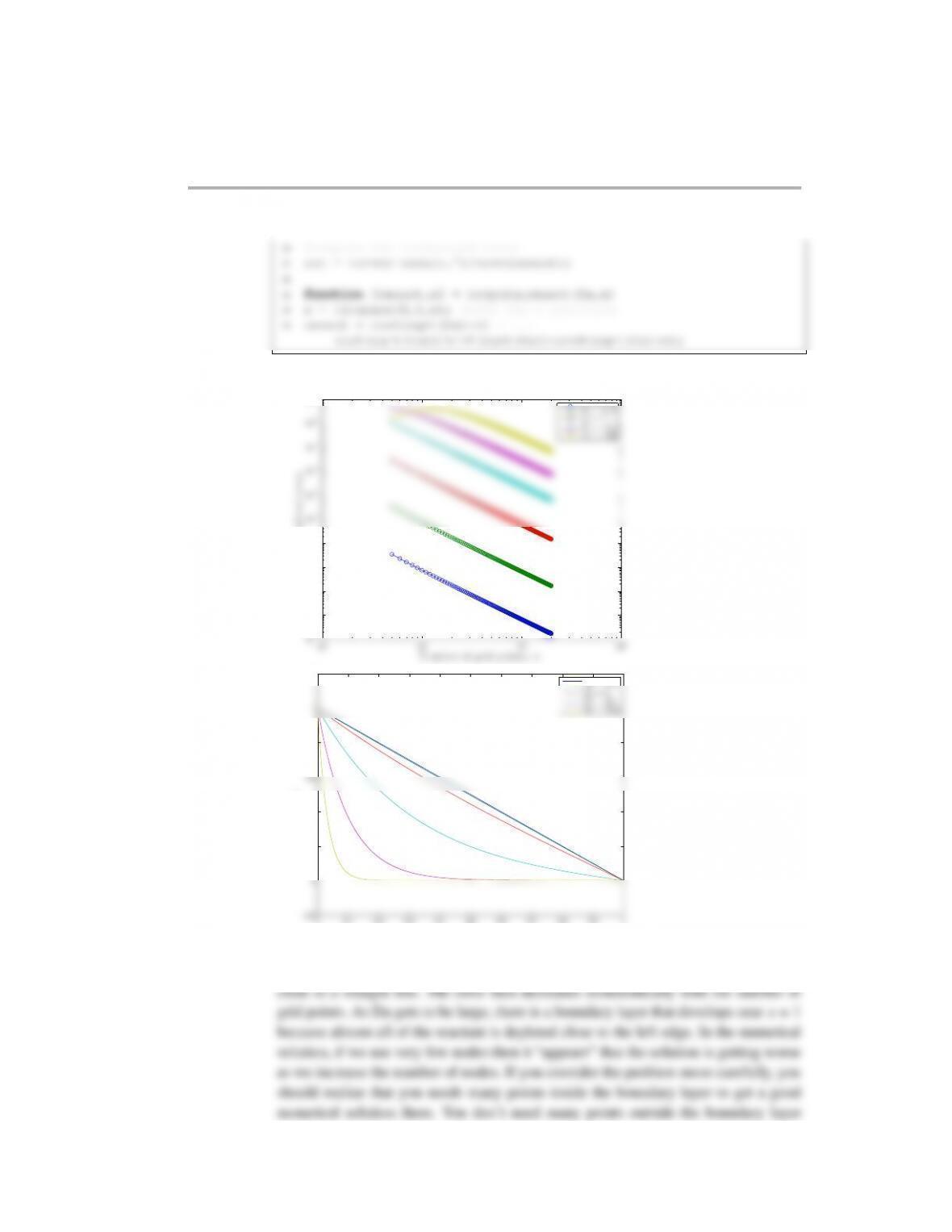
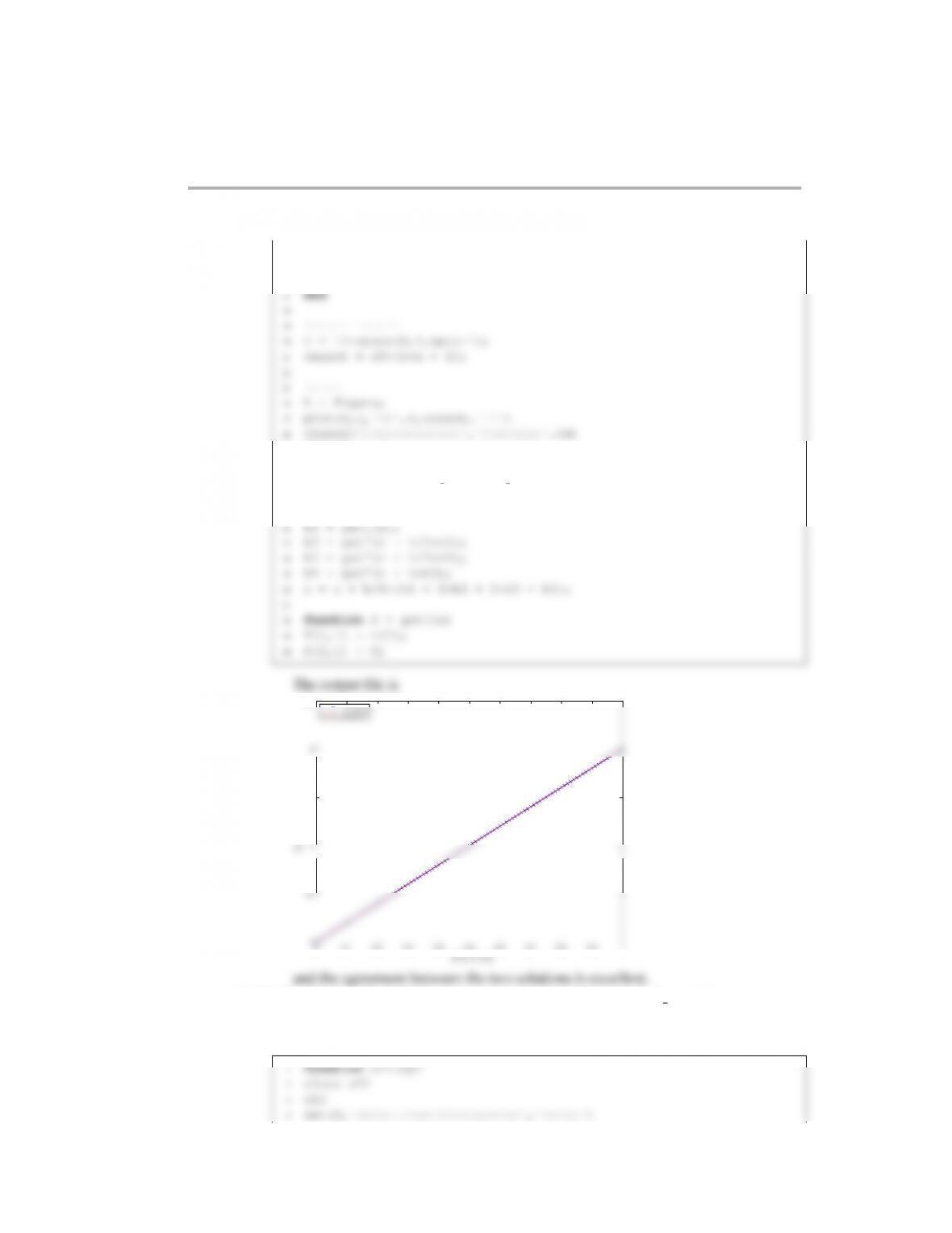
The output file is:
100101102103
10−11
10−10
10−9
10−8
10−7
10−6
10−5
10−4
10−3
10−2
10−1
N umb e r o f g r id p o int s , n
N or maliz e d e r r or
D a = 0 . 0 1
D a = 0 . 1
D a = 1
D a = 1 0
D a = 1 0 0
D a = 1 0 00
0 0.1 0.2 0.3 0.4 0.5 0.6 0.7 0.8 0.9 1
−0.2
0
0.2
0.4
0.6
0.8
1
1.2
x
c
D a = 0 . 0 1
D a = 0 . 1
D a = 1
D a = 1 0
D a = 1 00
D a = 1 00 0
The result for the accuracy is interesting from a numerical methods standpoint. For
Boundary value problems 367
since the concentration is almost zero there. If we use very few evenly spaced nodes,
(6.17) The files for this problem are contained in the folder s14c10p1 matlab. Integrating
once gives
dc
dx
=j
where jis a constant. Integrating again gives c=jx +c0, where c0=1 is the
The Matlab program is
1function s14c10p1
2clc
13
368 Boundary value problems
14 for i = 1:npts
15 z = RK4(z,dx);
16 c(i+1) = z(1);
27 xlabel(‘Position’,‘FontSize’,14)
28 legend(‘Numer’,‘Exact’,‘Location’,‘NorthWest’)
29 saveas(h,‘s14c10p1 solution figure.eps’,‘psc2’)
30
31 function z = RK4(z,h)
0 0.1 0.2 0.3 0.4 0.5 0.6 0.7 0.8 0.9 1
1
1.5
2
2.5
3
3.5
C on c e nt r at ion
Pos it ion
N u m e r
E x ac t
and the agreement between the two solutions is excellent.
(6.18) The files for this problem are contained in the folder s11c8p1 matlab.
Boundary value problems 369
5%loop through the values of dx for the problem and compute x(0)
0.001
9dxplot(i) = dx;
10 czero(i) = bvpsolve(dx);
11 end
12
23 n = 2/dx + 1;
24 xzero = 1/dx + 1; %location on the grid of x = 0
25 fprintf(‘Computing for n = %8d \t dx = %10.8f \t i = %8d …
\n’,n,dx,xzero)
26 A = zeros(n); b = zeros(n,1); %initialize the matrix problem
37 A(i,i) = -2*dt – 10*(1+sin(pi*x));
38 A(i,i+1) = dt;
39 xplot(i) = x;
40 end
41 c=A\b; %solve linear system
Boundary value problems 371
1function s15h10p1
2clc
3close all
4set(0,‘defaulttextinterpreter’,‘latex’)
15 %plot the two results
16 h = figure;
17 plot(x,c,‘ob’,x,c exact,‘-r’)
18 xlabel(‘$x$’,‘FontSize’,14)
19 ylabel(‘$c(x)$’,‘FontSize’,14)
30 [x,c] = solveBVP(dx,xmin,xmax);
31 c exact = exactSolution(dx,xmin,xmax);
32 err(i) = norm(c-c exact);
33 end
34 h = figure;
45 for i = 1:n
46 c exact(i) = cosh(x(i)) – q*sinh(x(i));
47 end
48
49 function [x,c] = solveBVP(dx,xmin,xmax)