Dynamical systems 325
72 function y = RK4(y0, h, Nt)
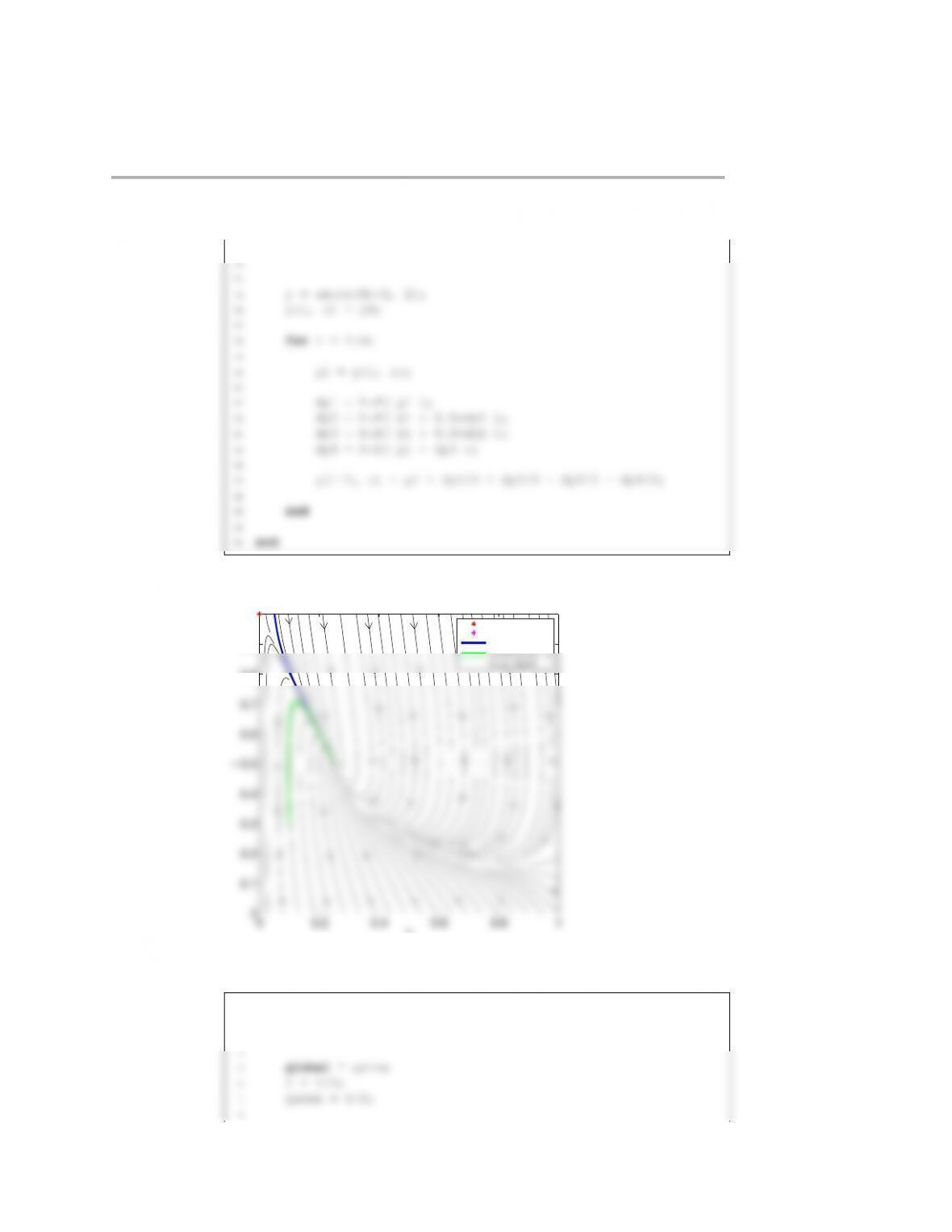
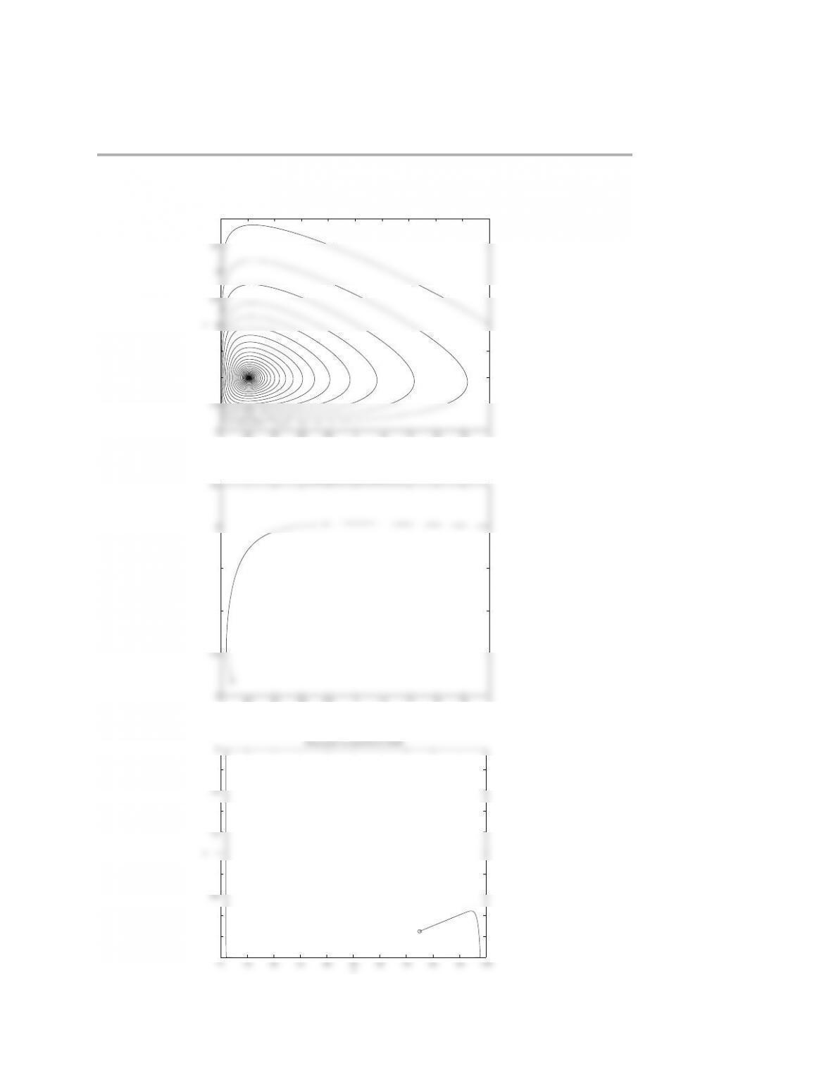
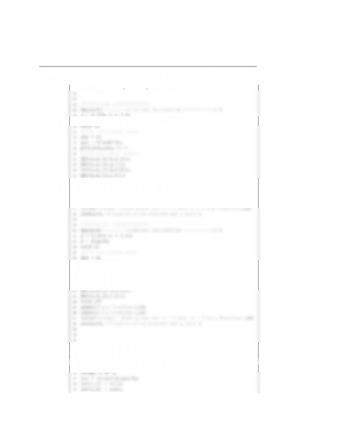
The phase plane plot is:
0 0.2 0.4 0.6 0.8 1
0
0.1
0.2
0.3
0.4
0.5
0.6
0.7
0.8
0.9
1
x
s
Solution to s13c9p123b
ss1
ss2
trajectory 1
trajectory 2
flow field
1function s13c9p123c()
2
3close all;
13 alpha = linspace(1.001, 2, n)’;
14 s2 = gamma ./ (alpha – 1);
15 x2 = Y*(1-s2);
16
17 % find out about stability, pick some points
27 L2 = eig(J2);
28 fprintf(‘%12f%12f%12f%12f%12f\n’,…
29 alpha(i), L1(1), L1(2), L2(1), L2(2));
30 end
31 fprintf(‘——————–———————-—\n’);
42 axis equal;
43 axis([1, 2, 0, 1]);
44 xlabel(‘$\alpha$’);
45 ylabel(‘x’);
46 legend(‘ss1’,‘ss2’);
57 text(0.5, 1.2, ‘Solution to s13c9p123c’);
58 saveas(gcf,‘s13c9p123 solution figure2.eps’,‘psc2’)
59
60 end
61
71 out(2, 1) = (-alpha .*s)./(Y .*(gamma + s));
72 out(2, 2) = -1 – ((alpha.*gamma.*x)./(Y.*(gamma + s).ˆ2));
73 end
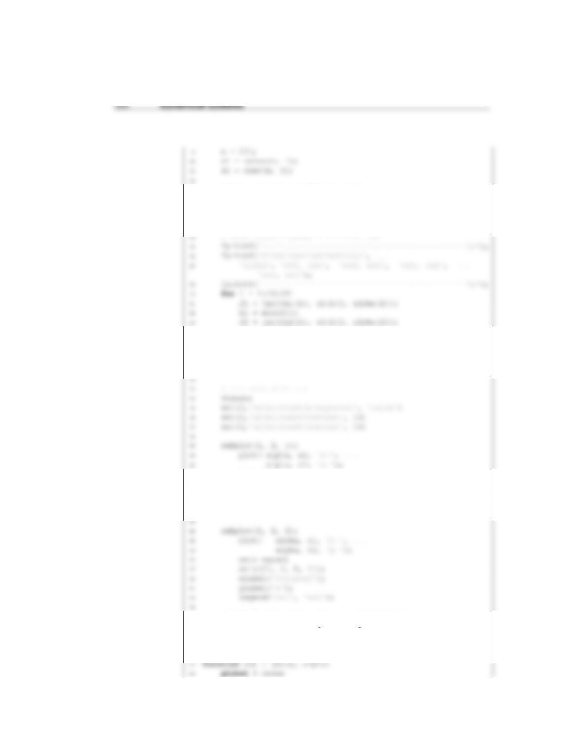
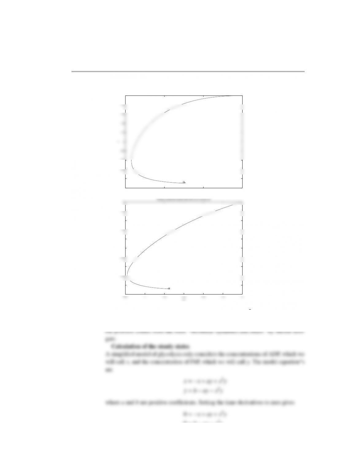
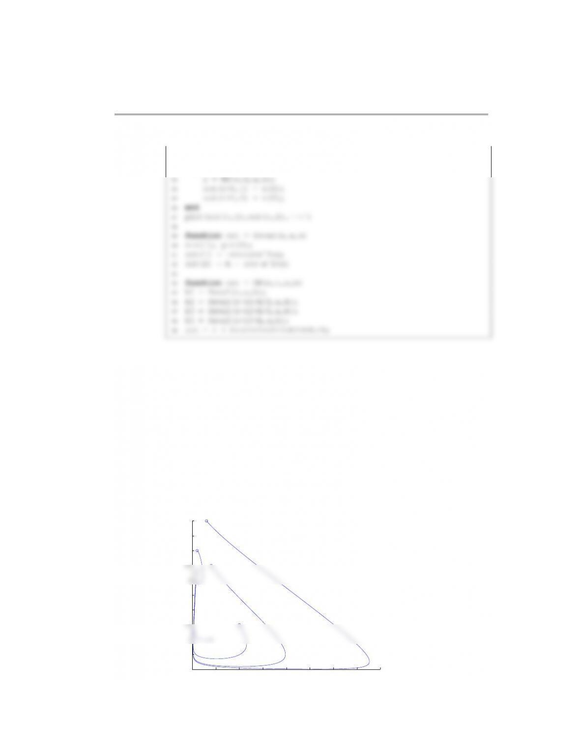
The bifurcation plot is:
1 1.5 2
0
0.2
0.4
0.6
0.8
1
α
x
ss1
ss2
1 1.5 2
0
0.2
0.4
0.6
0.8
1
α
s
S ol ut io n t o s 13 c 9p 12 3c
ss1
ss2
The output to the screen is:
1————————————————————
2alpha ev1, ss1 ev2, ss1 ev1, ss2 ev2, ss2
3————————————————————
(5.28) The files for this problem are contained in the folder s10cp2 matlab.
328 Dynamical systems
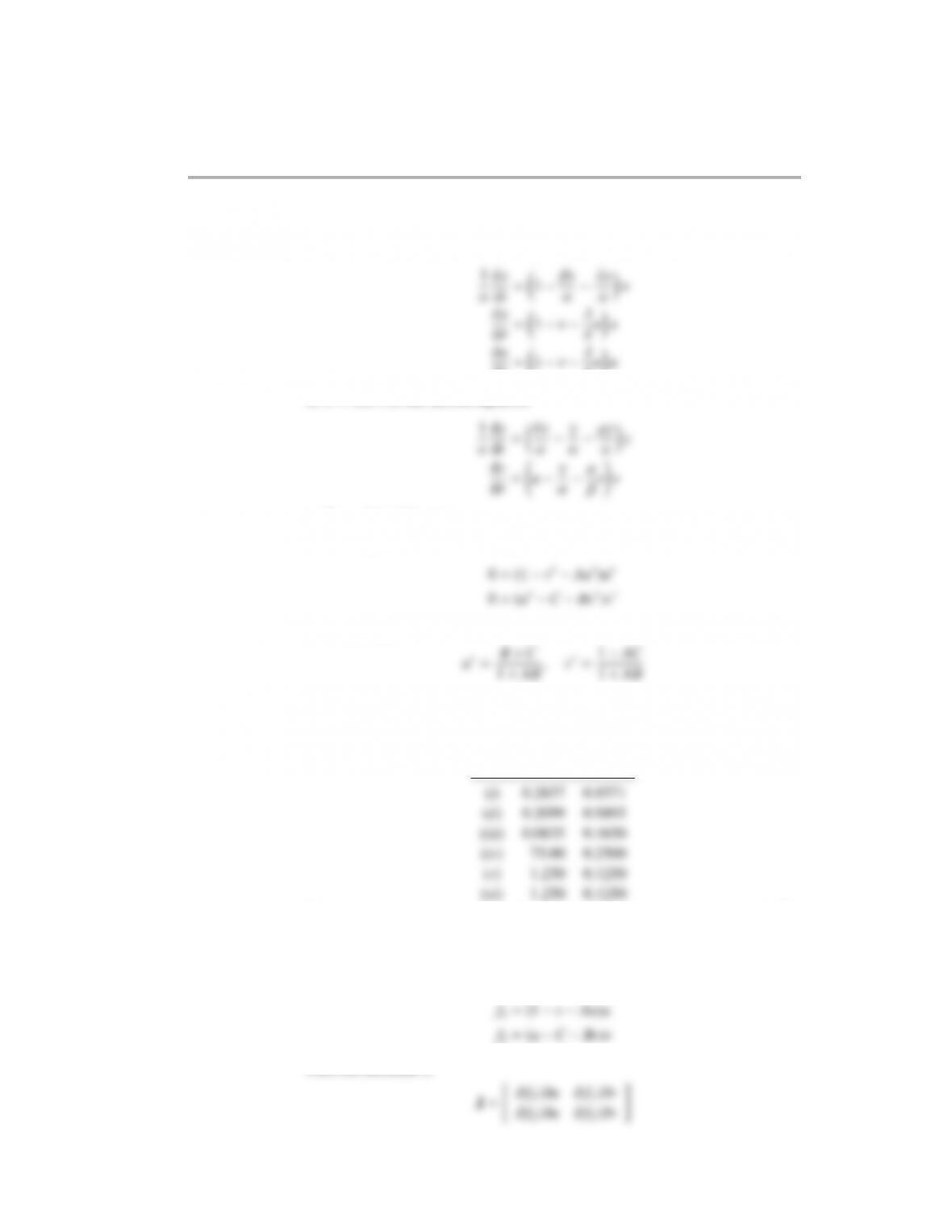
(a) With u=δx/α,v=βy/α and τ=αt, the first equation becomes:
dτ=1−v−λ
δuu
so A=λ/δ. For the second equation
so B=µ/β and C=γ/α.
(b) The steady state solutions correspond to
If we substitute
into these equation, then we get 0 =0 for both equations. In order for v∗≥0, we
required that AC <1.
(c) Substituting the values of A,B, and Cinto the particular steady states gives
u∗v∗
The ranges for the steady state solutions are 0 ≤u∗≤ ∞ and 0 ≤v∗≤1. The
Matlab program will automatically produce the steady state file and save it for
you.
(d) If we write the two equations as
Then the Jacobian is
Dynamical systems 329
which yields
To compute the eigenvalues, we need to solve det(J−λI) for the two roots of λ.
The results of this calculation are
λ1λ2type
(i) -0.1143 – 0.4940 i -0.1143 +0.4940 i stable spiral
(e) The Matlab code will produce the phase planes with the stable value of dt and
the number of oscillations pdisplayed in the title line.
The Matlab script for this problem is:
1function out=s10cp2(void)
2close all
3us=zeros(1,6); vs = zeros(1,6);
4for i = 1:6
5out = rk(i); %execute the program for the six cases
12 xlabel(‘u’), ylabel(‘v’), title(‘Steady states: x = 1, o = …
25 case 1
26 A = 0.5; B = 0.1; C = 0.2; %oscillatory
29 case 3
31 case 4
33 case 5
34 A = 0.7; B = 0.4; C = 1.2; %stable version with …
35 case 6
36 A = 0.7; B = 1.2; C = 1.1; %oscillatory version …
with stable point like case 5
37 end
%5.2f, C = %5.3f, dt = %6.3f \n’,A,B,C,dt)
43 fprintf(‘=================================================\n’)
44
45 % Set initial conditions
46 i = 1;
%6.4f\n’,us,vs)
61
62 % p is a counter that counts the number of times a cyclical …
%6.6f\n’,dt)
111 end
112 end
113 h = figure;
114 plot(u,v,‘k’,us,vs,‘ko’)
‘,num2str(p));
121 else
122 title graph = strcat(‘Phase plane for case …
‘,num2str(x),‘ with dt = ‘,num2str(dt));
332 Dynamical systems
132
133
134 function out = cp2f1(A,B,C,u,v)
138 out = (u-C-B*v)*v;
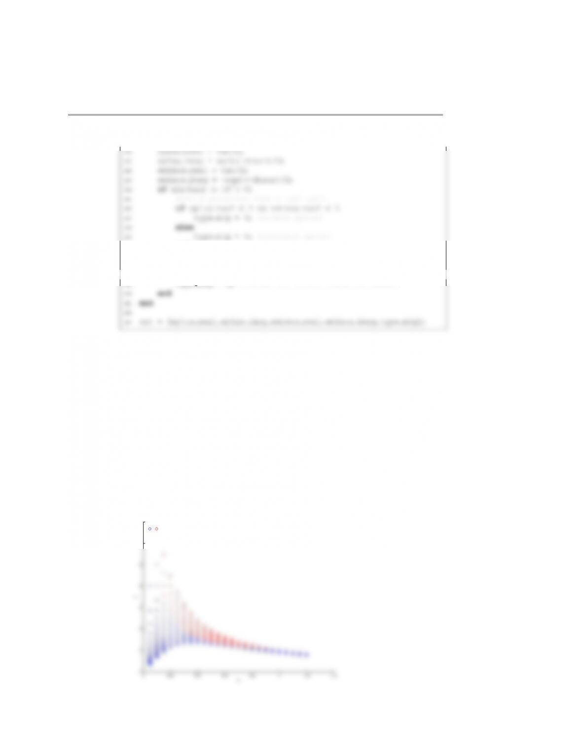
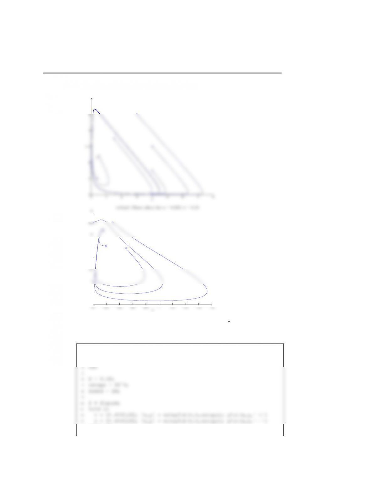
The output files are:
10−2 10−1 100101102
0.1
0.2
0.3
0.4
0.5
0.6
0.7
0.8
0.9
1
u
v
Steady states: x = 1, o = 2, * = 3, diamond = 4, square = 5, + = 6
0 0.2 0.4 0.6 0.8 1 1.2 1.4 1.6 1.8 2
0
0.5
1
1.5
2
2.5
3
Phase plane for case1 with dt =0.01 with p =5
u
v
Dynamical systems 333
0 0.2 0.4 0.6 0.8 1 1.2 1.4 1.6 1.8 2
0
0.5
1
1.5
2
2.5
3
3.5
4
Phase plane for case2 with dt =0.01 with p =62
u
v
0 0.2 0.4 0.6 0.8 1 1.2 1.4 1.6 1.8 2
0
0.5
1
1.5
2
2.5
Phase plane for case3 with dt =0.01
u
v
0 10 20 30 40 50 60 70 80 90 100
0
0.2
0.4
0.6
0.8
1
1.2
1.4
1.6
1.8
2
Phase plane for case4 with dt =0.005
u
v
334 Dynamical systems
0.5 1 1.5 2
0
0.2
0.4
0.6
0.8
1
1.2
1.4
1.6
1.8
2
Phase plane for case5 with dt =0.01
u
v
0.8 1 1.2 1.4 1.6 1.8 2
0
0.2
0.4
0.6
0.8
1
1.2
1.4
1.6
1.8
2
Phase plane for case6 with dt =0.01 with p =0
u
v
(5.29) The files for this problem are contained in the folder s11cp2 matlab.
This model was proposed by E.E. Sel’kov, “Self-oscillations in glycolysis. A sim-
ple kinetic model.” Eur. J. Biochem. 4, 79-86 (1968). The particular notation used in
Dynamical systems 335
Summing the equation*s gives x=b. Substitution back into the second equation*
and solving for ygives
Computing the Jacobian at steady state
−2b2
a+b2−(a+b2)
Computing the eigenvalues
Recall that the eigenvalues of a 2 ×2 system are
a+b2
Finding the boundary between the stable and unstable steady states
336 Dynamical systems
The case where τ=0 corresponds to
So there are going to be two values of bthat bound the stability envelope for a given
value of a. The point at which these two curves meet is going to be when the term in
the square root is zero, a=1/8, which corresponds to b=3/8.
The text of the output is also provided.
1function s11cp2 stability
2clc
3close all
4set(0,‘defaulttextinterpreter’,‘latex’)
14 for i = 1:npts a
15 a = (0.14/npts a)*i;
16 for j = 1:npts b
17 b = (1.2/npts b)*j;
18 xss = b;
28 for k = 5:9
29 output(curr row,k) = eigcal(k-4); %unpack the …
eigenvalue info
30 end
31
35 case 1
36 plot(xss,yss,‘ob’)
39 case 3
40 plot(xss,yss,‘ˆg’)
43 case 5
44 plot(xss,yss,‘xr’)
45 case 6
46 plot(xss,yss,‘kp’)
47 end
48 end
49 end
67 case 2
68 plot(a,b,‘or’)
71 case 4
72 plot(a,b,‘xb’)
75 case 6
76 plot(a,b,‘kp’)
77 end
78 end
79
89 for i = 1:npts
90 a = aplot(i);
91 %there are two values on the envelope for each value of a
92 b upper(i) = sqrt(0.5*(1-2*a+sqrt(1-8*a)));
93 b lower(i) = sqrt(0.5*(1-2*a-sqrt(1-8*a)));
104 saveas(h,‘s11cp2 solution figure2.eps’,‘psc2’)
105
106 dlmwrite(‘s11cp2 stability output.txt’,output)
107
108 out = 1;
117 delta = a + bˆ2; %determinant of Jacobian
118
119 discr = tauˆ2 – 4*delta; %discriminant of eigenvalues
120
121 if discr >= 0
132 type eig = 2; %unstable node
133 end
134 else
135 %the eigenvalues are complex
Dynamical systems 339
146 end
147 else
148 %the eigenvalues have no real part (to within …
round-off error)
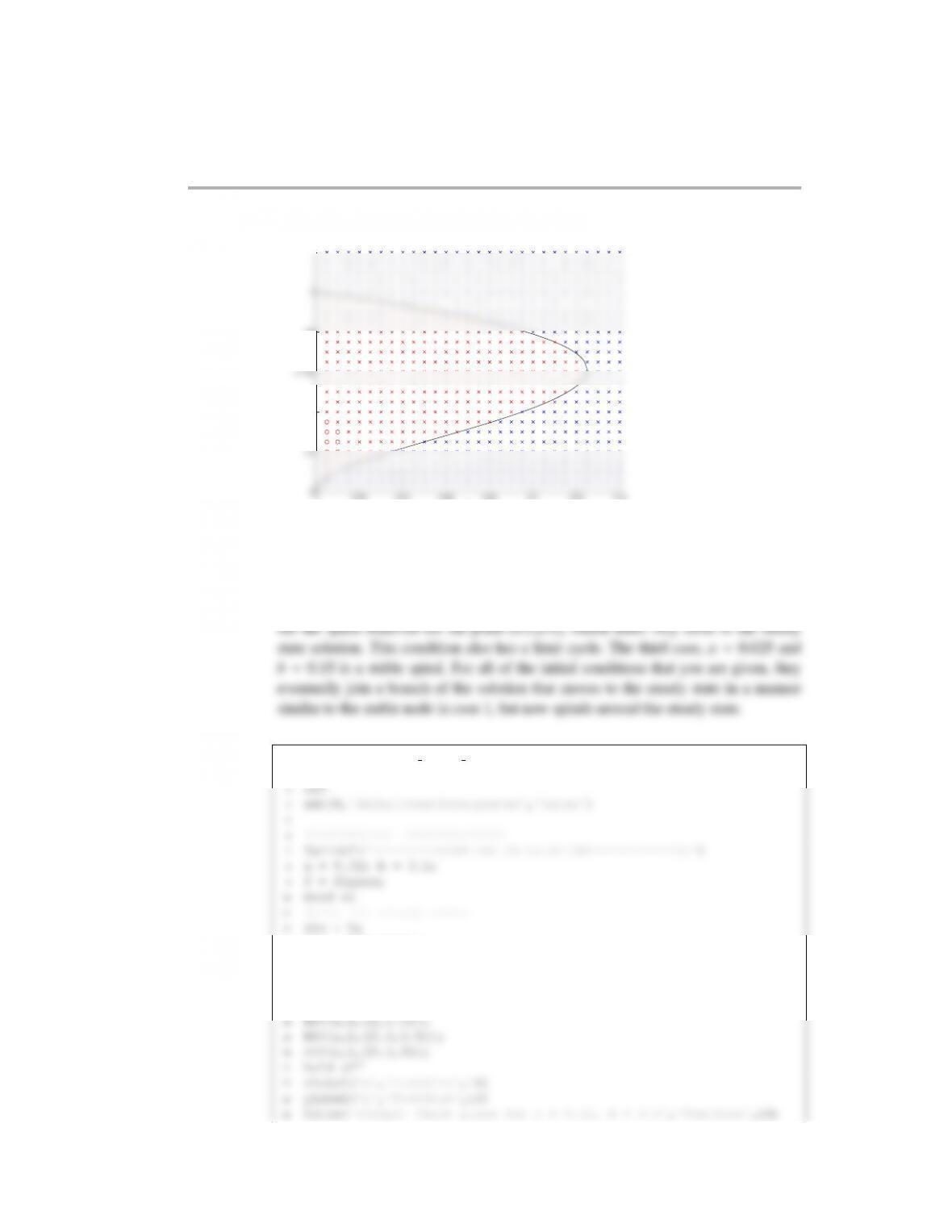
The output files are:
0 0.2 0.4 0.6 0.8 1 1.2 1.4
0
1
2
3
4
5
6
7
x
y
s 11c p 2: S t e ad y s ta t e c l as s ifi c at i on
340 Dynamical systems
0 0.02 0.04 0.06 0.08 0.1 0.12 0.14
0
0.2
0.4
0.6
0.8
1
a
b
s 11c p 2: S ta bi li ty e nv e lo pe
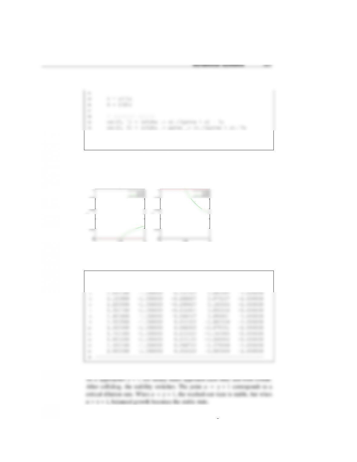
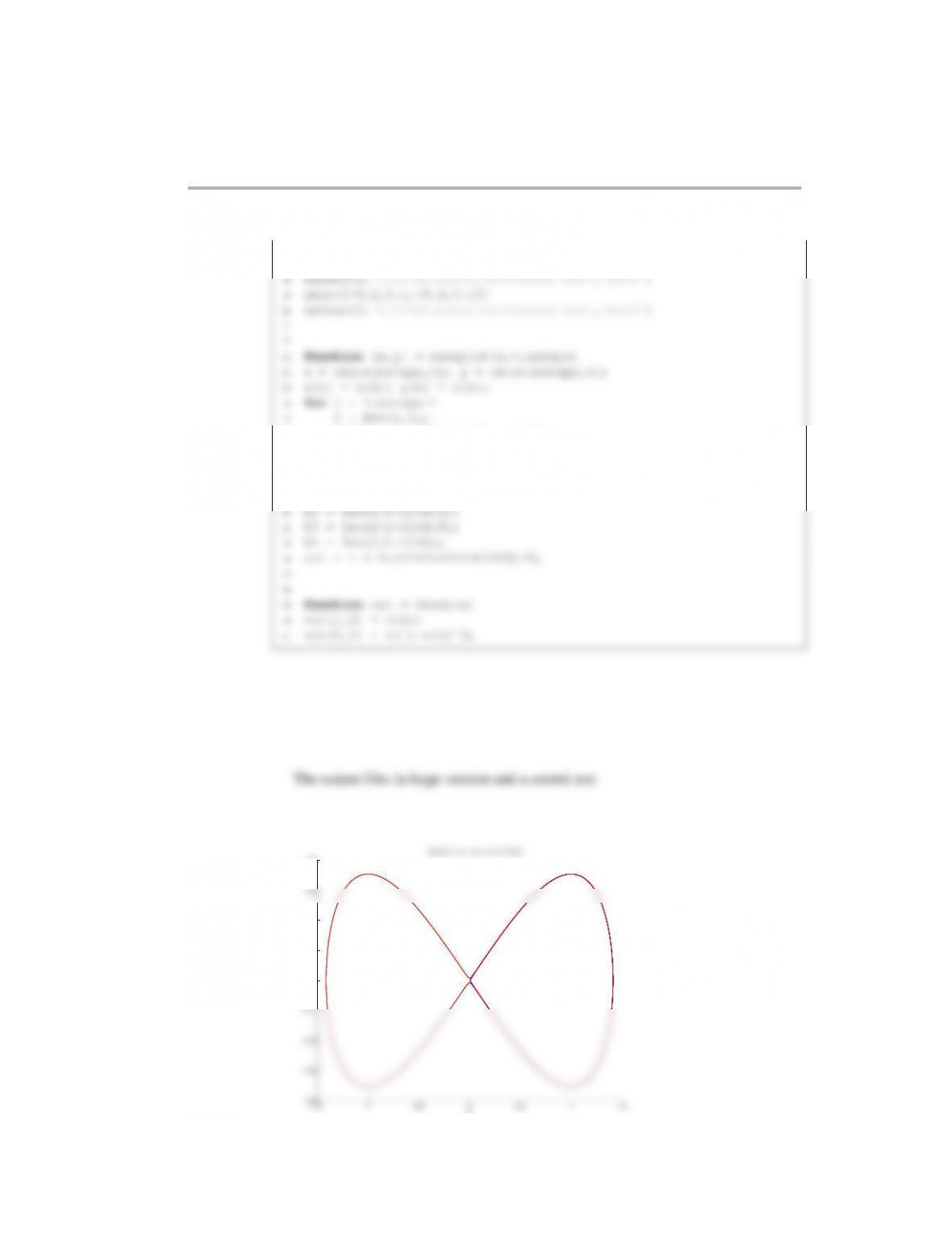
Phase planes
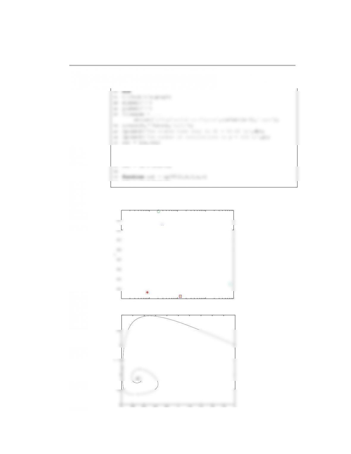
The Matlab code and the resulting phase planes are below. The first case, a=0.02
and b=0.1 corresponds to a stable node. Although the initial condition (0.1,4) looks
like it is curving and might be a spiral, it goes straight to the steady state so it is still
a stable node. The second case, a=0.015 and b=0.4, is an unstable spiral. You can
1function s11cp2 phase plane
2close all
13 yss = b/(a+bˆ2);
14 plot(xss,yss,‘xr’)
15 %plot the other values
16 RK4(a,b,[0.1,4]);
17 RK4(a,b,[0.4,1]);
Dynamical systems 341
25 saveas(f,‘s11cp2 solution figure3.eps’,‘psc2’)
31 f = figure;
42 RK4(a,b,[4,3]);
43 RK4(a,b,[3,5]);
44 hold off
45 xlabel(‘x’,‘FontSize’,14)
46 ylabel(‘y’,‘FontSize’,14)
57 yss = b/(a+bˆ2);
58 plot(xss,yss,‘xr’)
59 %plot the other values
60 RK4(a,b,[0.5,2.4]);
61 RK4(a,b,[0.2,2.5]);
72
73 function out = RK4(a,b,z)
74 fprintf(‘Computing for a = %4.3f, b = %3.2f, x0 = %3.2f and y0 …
= %3.2f\n’,a,b,z(1),z(2))
75 h = 0.01;
342 Dynamical systems
80 plot(z(1),z(2),‘ob’)
81
82 for i = 1:nsteps
The output files are:
0 0.5 1 1.5 2 2.5 3 3.5 4
0
0.5
1
1.5
2
2.5
3
3.5
4
4.5
5
x
y
sc 11p2: P has e plane f or a = 0.02, b = 0.1
Dynamical systems 343
0 1 2 3 4 5 6 7 8
0
1
2
3
4
5
6
x
y
sc 11p2: P hase plane f or a = 0.015, b = 0.4
0 0.2 0.4 0.6 0.8 1 1.2 1.4 1.6 1.8
0
0.5
1
1.5
2
2.5
3
3.5
4
x
y
sc 11p2: Phas e plane for a = 0.025, b = 0.15
(5.30) The files for this problem are contained in the folder s11c7p1 matlab.
The Matlab script is:
1function s11c7p1
2close all
3set(0,‘defaulttextinterpreter’,‘latex’)
14 hold off
15 xlabel(‘x’,‘FontSize’,14)
344 Dynamical systems
16 ylabel(‘v’,‘FontSize’,14)
17 title(‘Solution to s11c7p1’,‘FontSize’,14)
28 x(j+1) = z(1); y(j+1) = z(2);
29 end
30
31 function out = RK4(z,h)
32 k1 = feval(z);