Dynamical systems 305
2clc
3close all
4set(0,‘defaulttextinterpreter’,‘latex’)
5
16
17 xlabel(‘$x 1$’,‘FontSize’,14)
18 ylabel(‘$x 2$’,‘FontSize’,14)
19
20 saveas(h,‘s12c9p3 solution figure.eps’,‘psc2’)
31 for i = 1:nsteps
32 x = RK4(x,h);
33 x1(i+1) = x(1);
34 x2(i+1) = x(2);
35 end
46 function out = feval(x)
47 mu = 1.1;
48 out(1) = x(2);
49 out(2) = mu*(1-x(1)ˆ2)*x(2)-x(1);
The output file is:
-1 0 -1 Neutrally stable (no classification)
2 4.2287 -2.2287 Saddle point
3 1.5+4.7838ı1.5−4.7838ıUnstable focus
(b) The program below uses RK4 to construct the phase plane:
1function s14c9p2
2clc
12 title text = ‘Global Plot’;
13 makeplot(xmax,xmin,ymax,ymin,title text,15)
14
15 ymax = -2.5;
16 ymin = -3.5;
27 title text = ‘Steady state at (0,-1)’;
28 makeplot(xmax,xmin,ymax,ymin,title text,8)
29
30 ymax = ymax+1;
31 ymin = ymin+1;
308 Dynamical systems
42 title text = ‘Steady state at (0,2)’;
43 makeplot(xmax,xmin,ymax,ymin,title text,8)
44
45 ymax = ymax+1;
55 disp(title text)
56 fprintf(‘\n’)
57 h = figure;
58 hold on
59 for i = 1:npts
70 ylabel(‘$y$’,‘FontSize’,14)
71 title(title text,‘FontSize’,14)
72 saveas(h,strcat(title text,‘.eps’),‘psc2’)
73
74 function [xout,yout] = get trajectory(x,y)
83 xout(1) = x;
84 yout(1) = y;
85 z = [x;y]; %put into a vector
86
87 for i = 2:nsteps+1
96 %autonomous
97 k1 = feval(z);
98 k2 = feval(z + 0.5*h*k1);
99 k3 = feval(z + 0.5*h*k2);
100 k4 = feval(z + h*k3);
101 z=z+h/6*(k1 + 2*k2 + 2*k3 + k4);
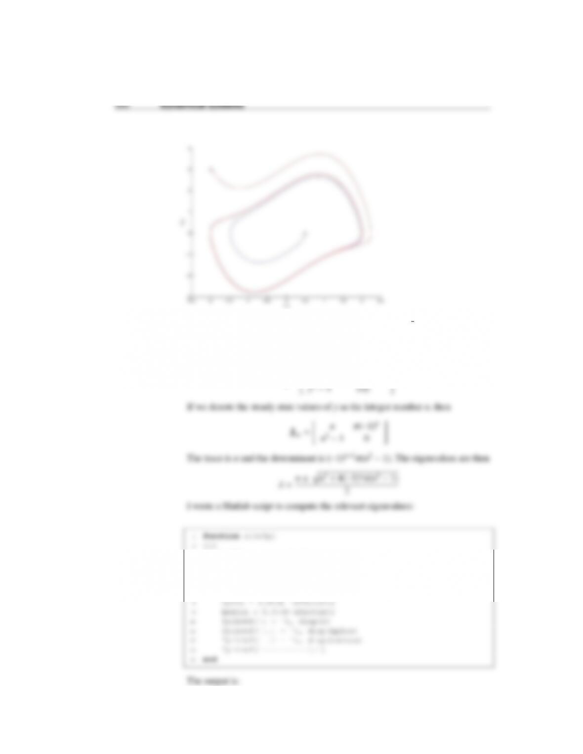
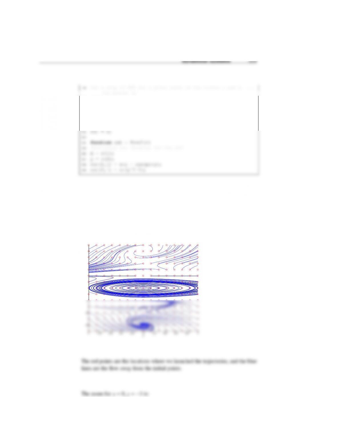
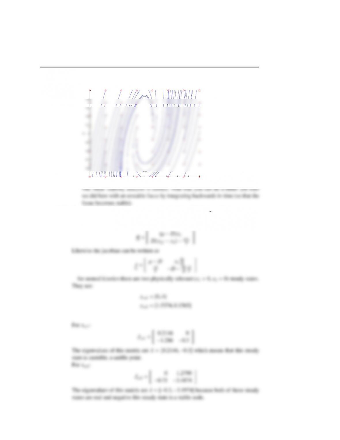
The global phase plane is:
−1 −0.8 −0.6 −0.4 −0.2 0 0.2 0.4 0.6 0.8 1
−3
−2
−1
0
1
2
3
x
y
Global P lot
310 Dynamical systems
−1 −0.8 −0.6 −0.4 −0.2 0 0.2 0.4 0.6 0.8 1
−3.5
−3.4
−3.3
−3.2
−3.1
−3
−2.9
−2.8
−2.7
−2.6
−2.5
x
y
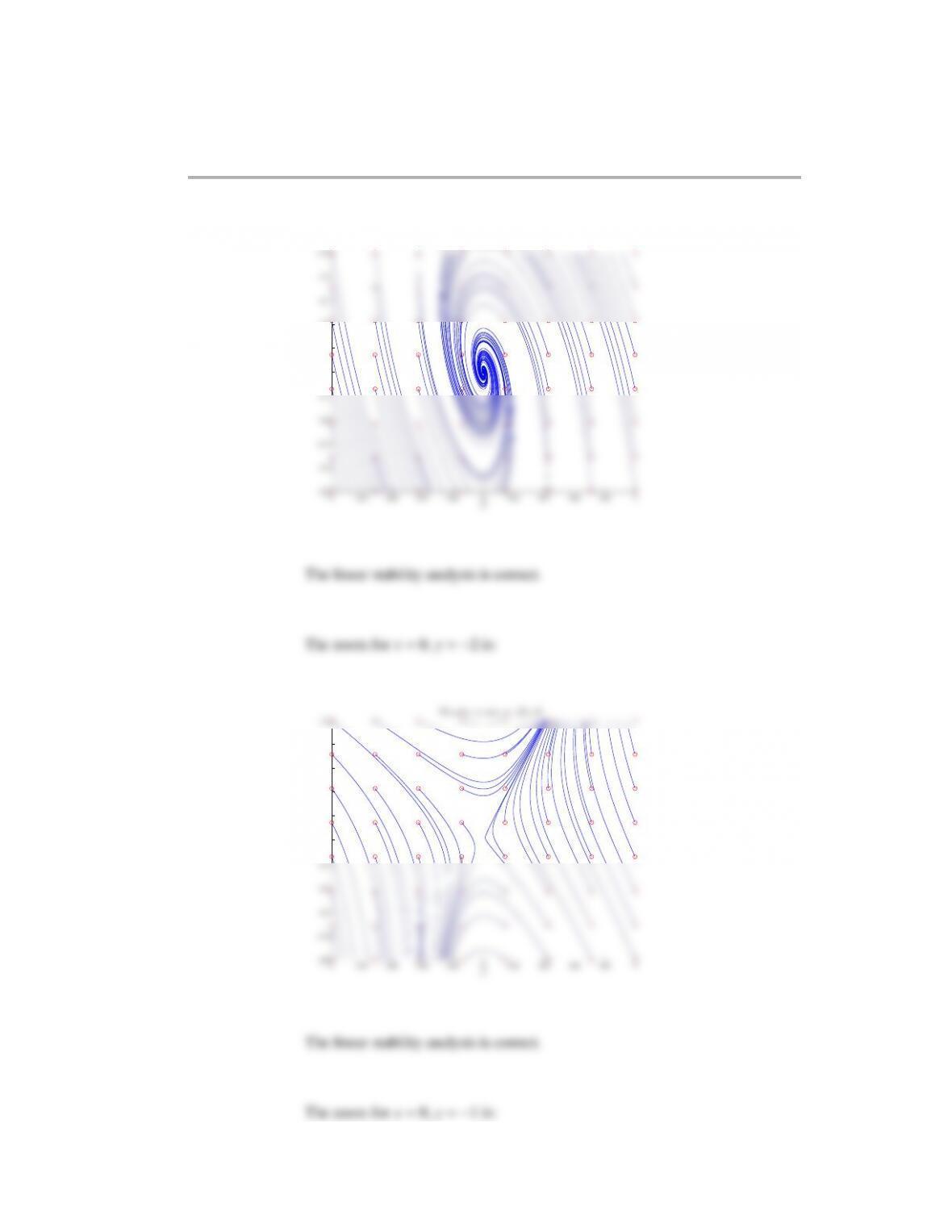
Ste ady stat e at (0,–3)
x
312 Dynamical systems
−1 −0.8 −0.6 −0.4 −0.2 0 0.2 0.4 0.6 0.8 1
0.5
0.6
0.7
0.8
0.9
1
1.1
1.2
1.3
1.4
1.5
x
y
Ste ady st ate at (0,1)
The zoom for x=0, y=3 is:
Dynamical systems 313
−1 −0.8 −0.6 −0.4 −0.2 0 0.2 0.4 0.6 0.8 1
2.5
2.6
2.7
2.8
2.9
3
3.1
3.2
3.3
3.4
3.5
x
y
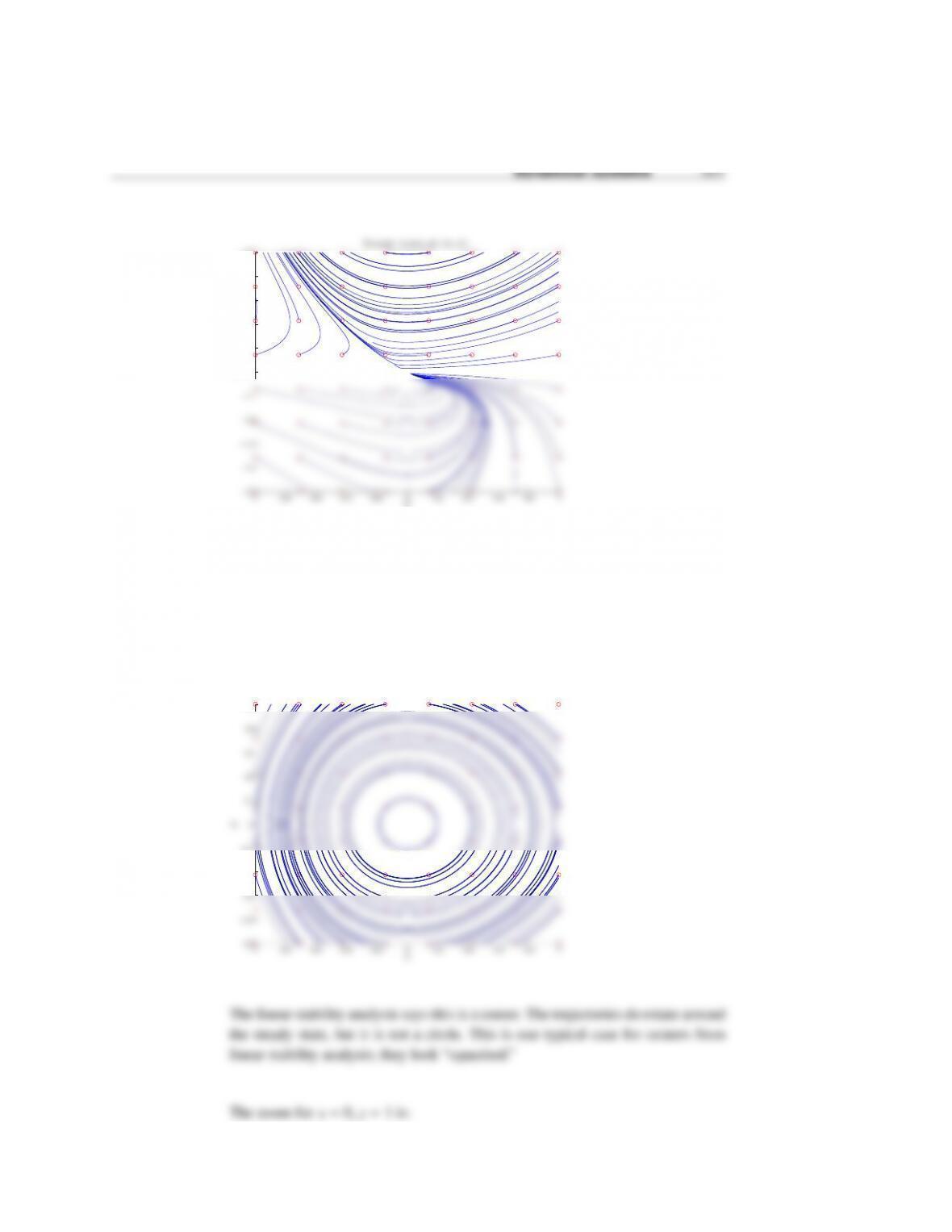
Ste ady st ate at (0,3)
(5.23) The files for this problem are contained in the folder f08c8p2 matlab
Newton-Raphson will be used to calculate the steady state values. In general the
residual vector can be written as:
314 Dynamical systems
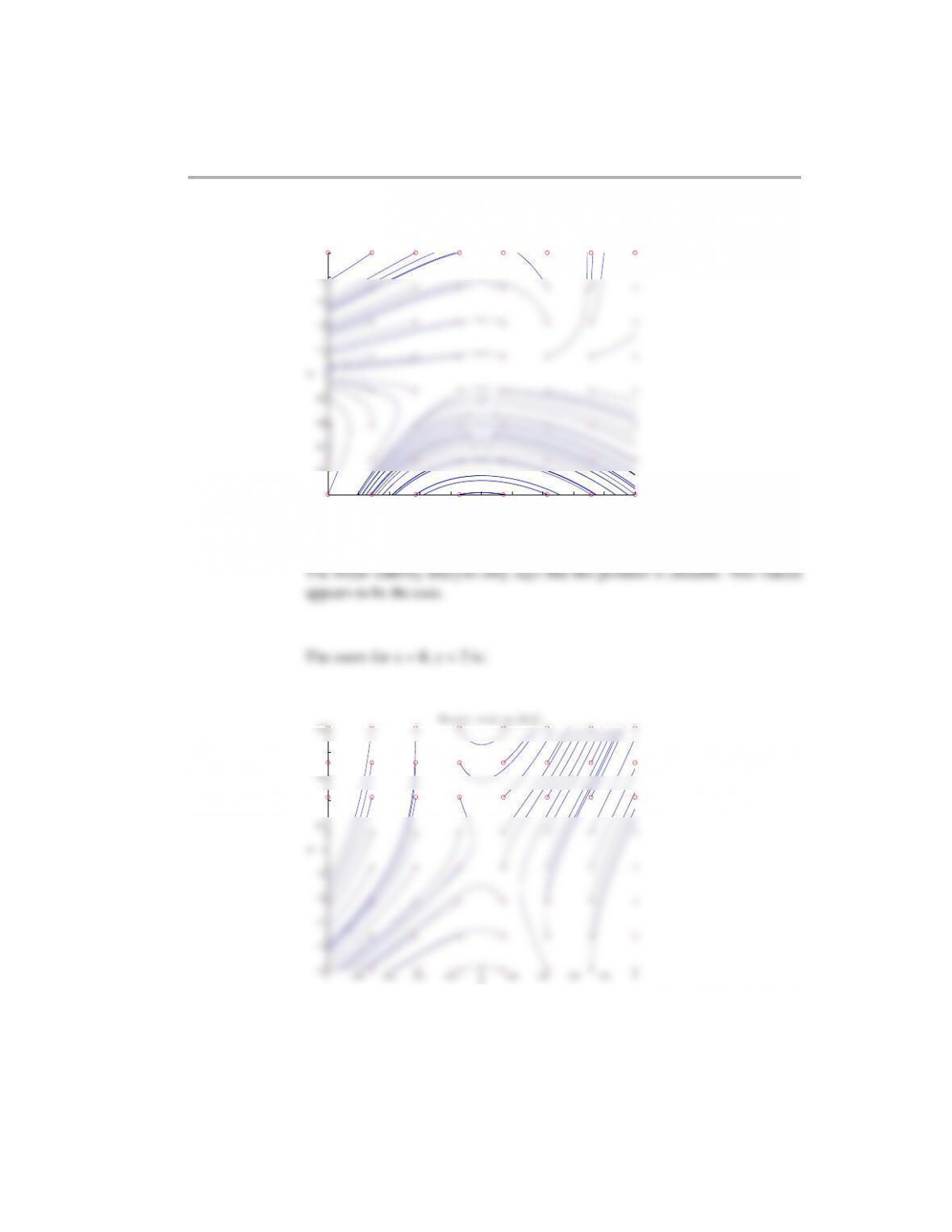
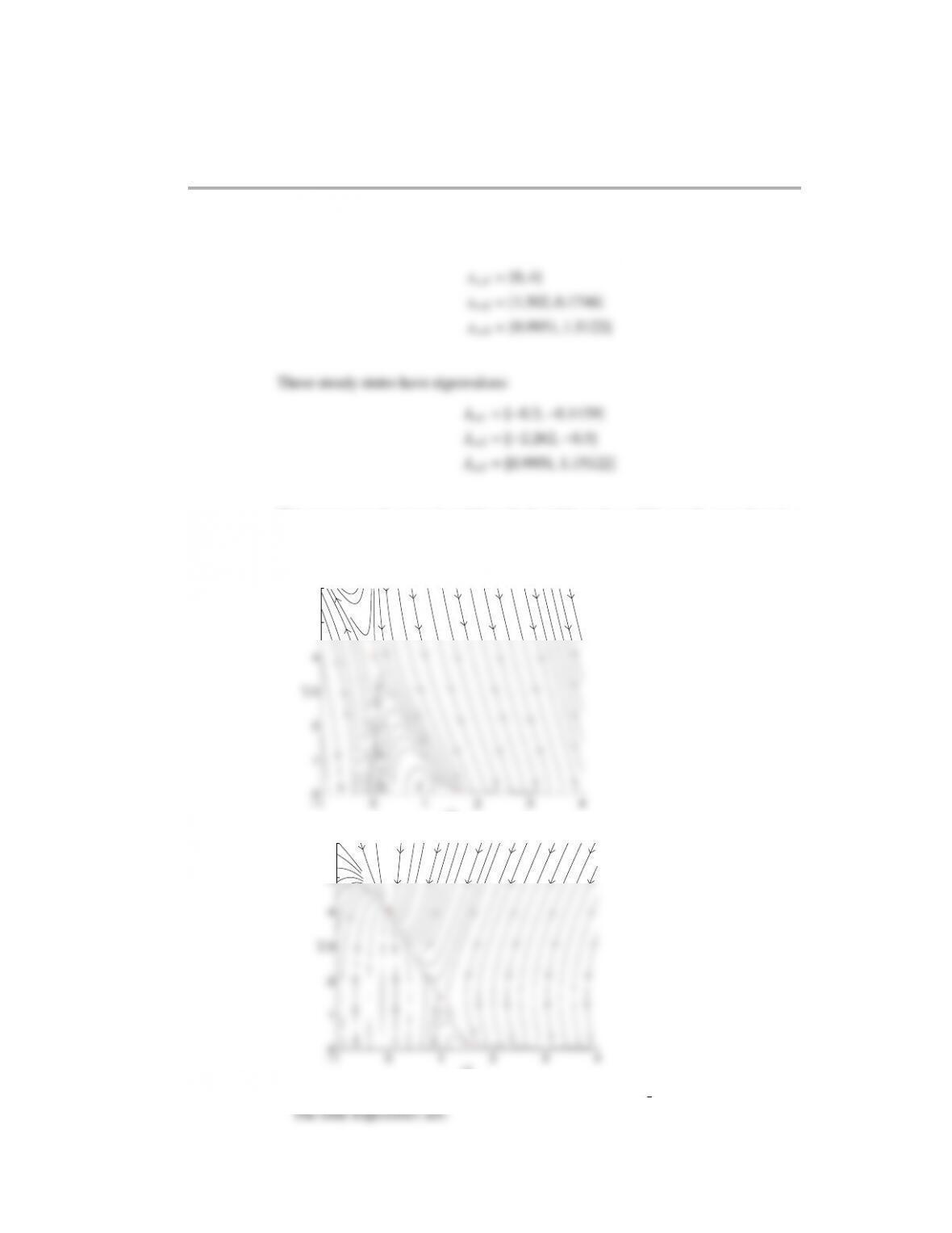
For substrate inhibition there are three relevant steady states at:
This means steady states 1 and 2 are both stable nodes, while steady state three is a
saddle point and therefor unstable.
The phase planes are:
−1 0 1 2 3 4
0
1
2
3
4
5
6
Phase Plane for Monod Kinetics
x1
x2
−1 0 1 2 3 4
0
1
2
3
4
5
6
Phase Plane for Substrate Inhibition
x1
x2
(5.24) The Matlab code for this problem can be found in f08c9p1 matlab.
Dynamical systems 315
0 5 10 15 20 25 30
0.5
1
1.5
2
2.5
3
3.5
4
4.5
5
5.5
Predator-Prey Population Curves RK4
Time
Population
Prey
Predator
0 5 10 15 20 25 30
0
1
2
3
4
5
6
7
8
9
10
Predator-Prey Population Curves EE
Time
Population
Prey
Predator
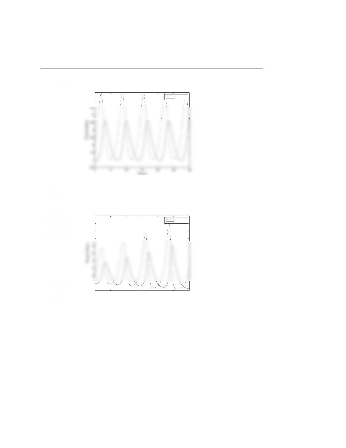
The Explicit Euler integration shows oscillations of increasing amplitude in both
predator and prey numbers. This suggests that the system in unstable. The Runge-
Kutta system however does not share this instability so it must be attributed to the
method not the system.
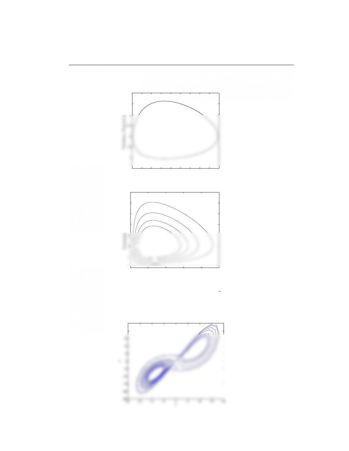
The instability of EE is confirmed by the phase plot, while RK is shown to be
stable.
316 Dynamical systems
1 1.5 2 2.5 3 3.5 4 4.5 5 5.5
0.5
1
1.5
2
2.5
3
3.5
4
Predator-Prey Phase Plane RK4
Prey Population
Predator Population
0 2 4 6 8 10
0
1
2
3
4
5
6
7
Predator-Prey Phase Plane EE
Prey Population
Predators Population
(5.25) The files for this problem can be found in f08c9p2 matlab
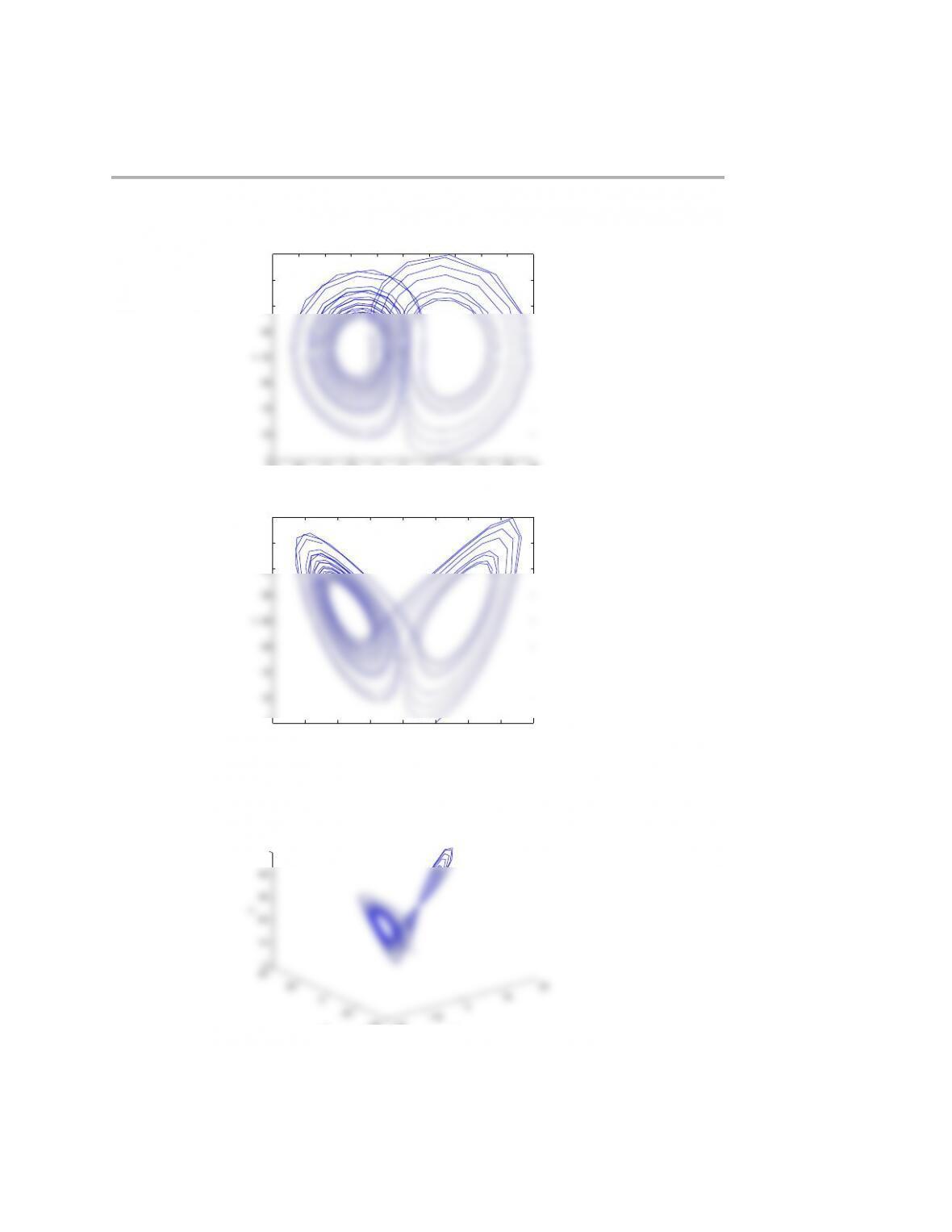
(a) For the given initial conditions the phase planes are
−20 −15 −10 −5 0 5 10 15 20
−25
−20
−15
−10
−5
0
5
10
15
20
25
x−y Phase Plane
x
y
Dynamical systems 317
−25 −20 −15 −10 −5 0 5 10 15 20 25
5
10
15
20
25
30
35
40
45
y−z Phase Plane
y
z
−20 −15 −10 −5 0 5 10 15 20
5
10
15
20
25
30
35
40
45
x−z Phase Plane
x
z
The 3 dimensional plot is
−20
−10
0
10
20
−40
−20
0
20
40
0
10
20
30
40
50
x
x−y−z Phase Plane
y
z
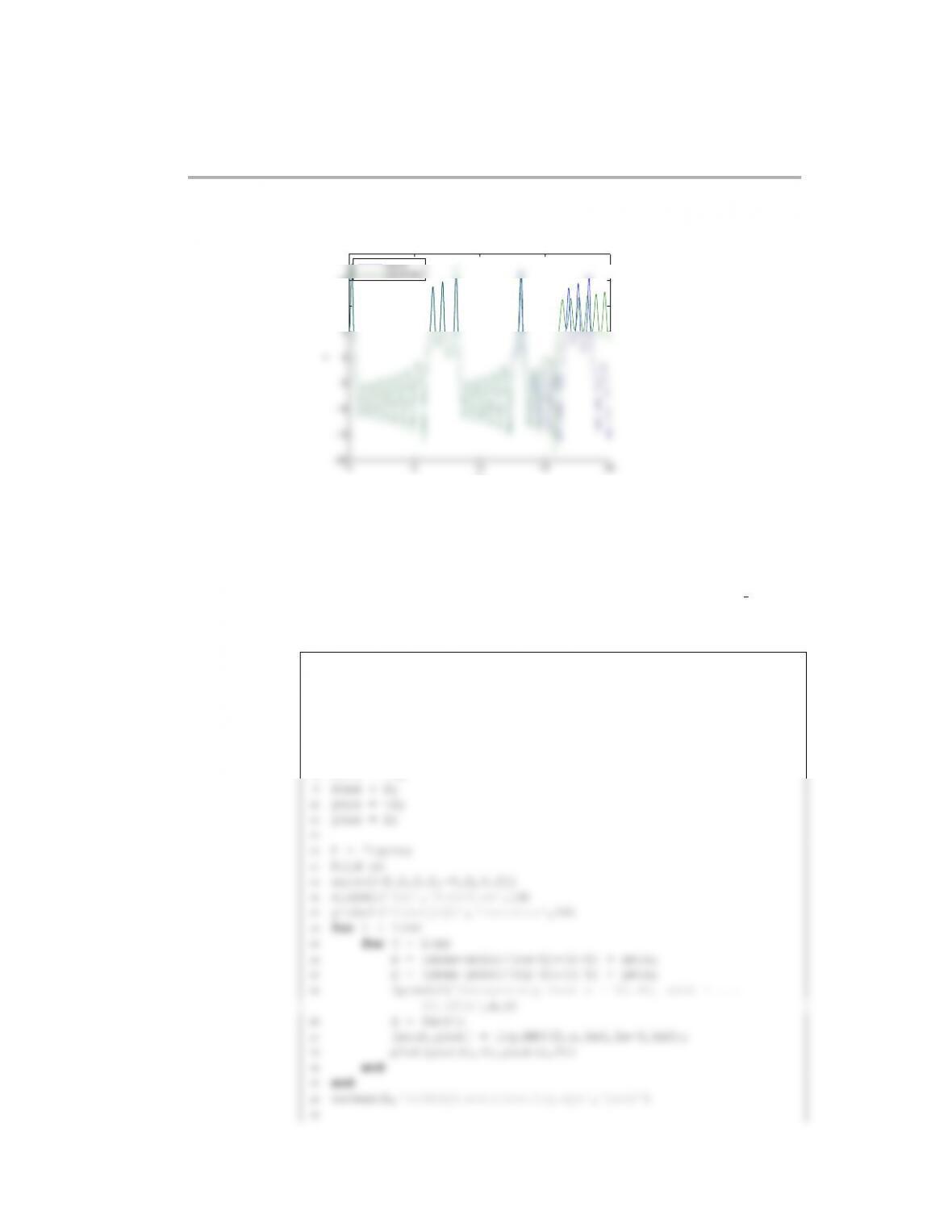
(b) The two trajectories are shown on the graph below. Based on the graph the sys-
in the solution starting around t=13
318 Dynamical systems
0 5 10 15 20
−20
−15
−10
−5
0
5
10
15
20
Time trajectory for two initial conditions in x
t
x
x(0)=5
x(0)=5.001
(5.26) The problem we are studying here is called the Duffing oscillator and it is a classic
problem in chaos theory. There is a nice introduction to the problem at http://www.
scholarpedia.org/article/Duffing\_oscillator and this article has links to
classic references on the problem.
(a) The files to solve this problem are contained in the directory s15c9p2 matlab.
The Matlab program to solve this problem is
1function s15h9p2
2clc
3close all
4set(0,‘defaulttextinterpreter’,‘latex’)
5
6nx = 10;
7ny = 10;
8xmin = -2;
Dynamical systems 319
30
31
32
33 function [xout,yout] = ivp RK4(x0,y0,n,h,i out)
34 % x0 = initial value for x
35 % y0 = initial value for y
36 % n = number of steps to take
37 % h = step size
45 for i = 1:n
46 k1 = getf(x,y);
47 k2 = getf(x + 0.5*h,y + 0.5*h*k1);
48 k3 = getf(x + 0.5*h,y + 0.5*h*k2);
49 k4 = getf(x + h, y + h*k3);
55 yout(count,:) = y;
56 end
57 end
58
59 function out = getf(x,y)
The program uses RK4 to make the phase plane for points in the interval [−2,2]
for both variables. This is sufficient to solve the problem. There is nothing spe-
cial that you need to do to implement RK4, so you do not need to provide any
equations here. All you needed to do was set the equation to
and use the standard algorithm for systems of equations.
The output file is
320 Dynamical systems
−2 −1.5 −1 −0.5 0 0.5 1 1.5 2
−4
−3
−2
−1
0
1
2
3
4
x
˙x
The result agrees with the phase plane analysis from Problem ?. There is a saddle
at the origin and two stable spirals at x=±2/3 and zero velocity.
(b) The files to solve this problem are contained in the directory s15c9p3 matlab.
We need to modify the equations for the forcing function to
x
t
˙x
1
The Matlab file to solve this problem is
1function s15h9p3
2clc
3close all
4set(0,‘defaulttextinterpreter’,‘latex’)
5
14 xlabel(‘$x$’,‘FontSize’,14)
15 ylabel(‘$\dot{x}$’,‘FontSize’,14)
16
17 x = -1; y = -1;
18 fprintf(‘Integrating from x = %6.4f, xdot = %6.4f\n’,x,y)
19 z = [x;y;0];
Dynamical systems 321
27 fprintf(‘Integrating from x = %6.4f, xdot = %6.4f\n’,x,y)
28 z = [x;y;0];
42 % h = step size
43 % i out = values to output x and y to [xout, yout]
44 % requires the function getf(x,y)
45 nout = ceil(n/i out); %number of output values
46 count = 1; %number of outputs used
47 xout = zeros(nout,1); xout(1) = x0;
48 yout = zeros(nout,3); yout(1,:) = y0;
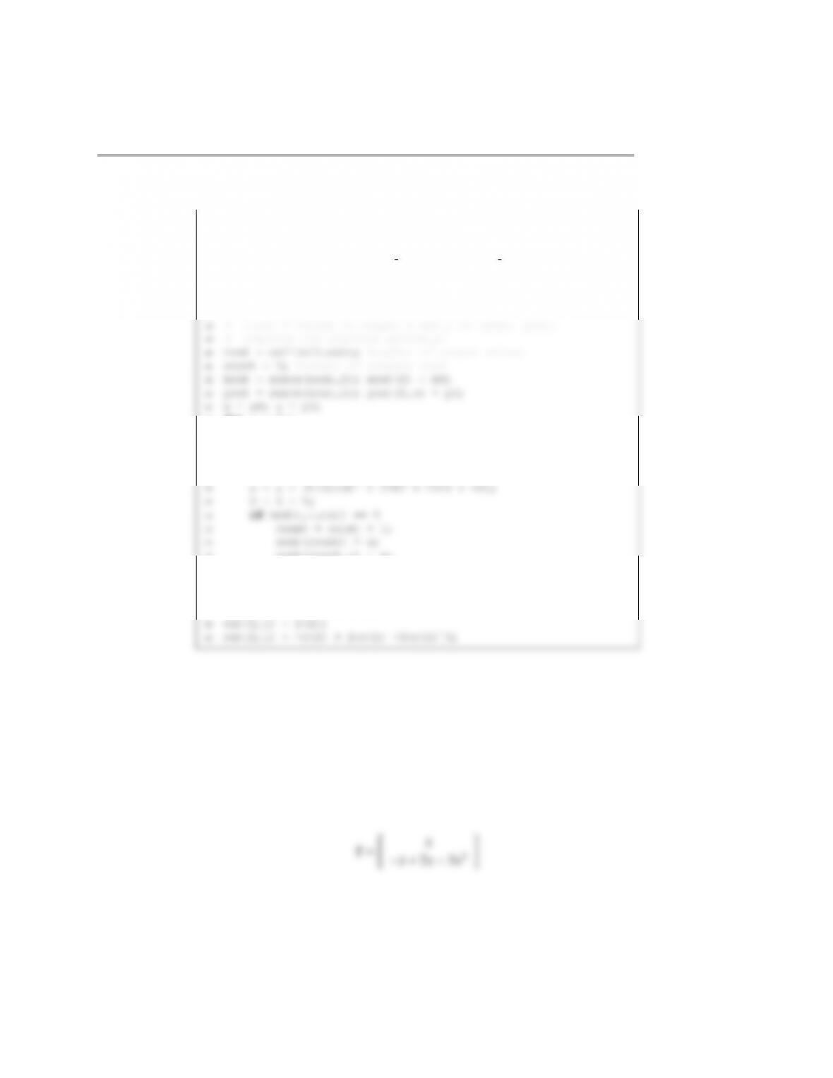
The output file is
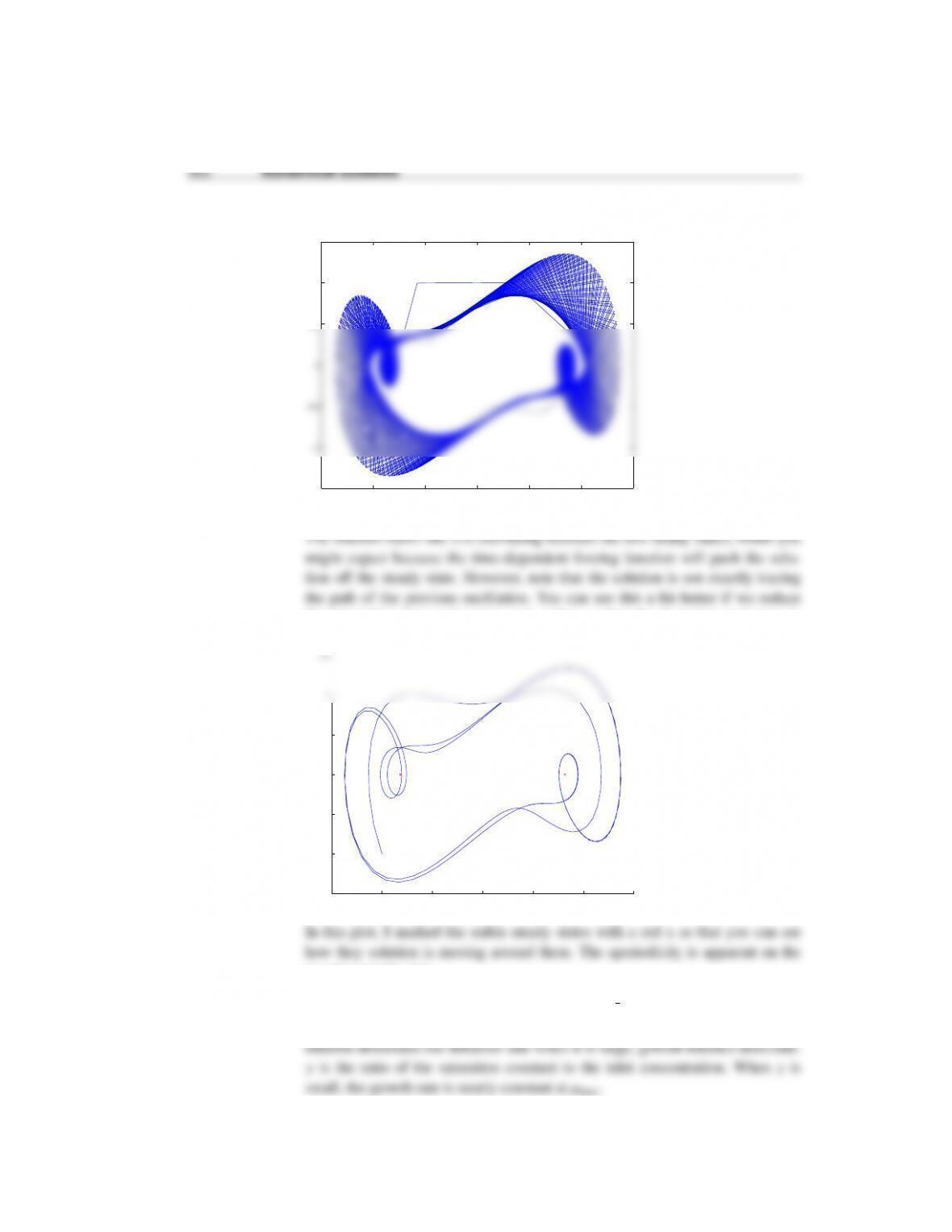
−1.5 −1 −0.5 0 0.5 1 1.5
−1.5
−1
−0.5
0
0.5
1
1.5
This is called aperiodic behavior, and it is a characteristic of chaotic systems.
the integration time and output more points so that the short-time trajectory is
smooth:
−1.5 −1 −0.5 0 0.5 1 1.5
−1.5
−1
−0.5
0
0.5
1
1.5
x
˙x
negative steady state.
(5.27) The files for this problem are in the folder s13c9p123 matlab.
(a) 1. αis the ratio of maximum growth rate to dilution rate. When αis small,
2. There are two steady states. One corresponds to “wash-out” when the dilution
Dynamical systems 323
rate large and dominates the growth kinetics
3. Using y=[x,s]Tin dy
dt
=f(y)
αs
γ+s
−1αγx
(γ+s)2
Y(γ+s)−1−αγx
Y(γ+s)2
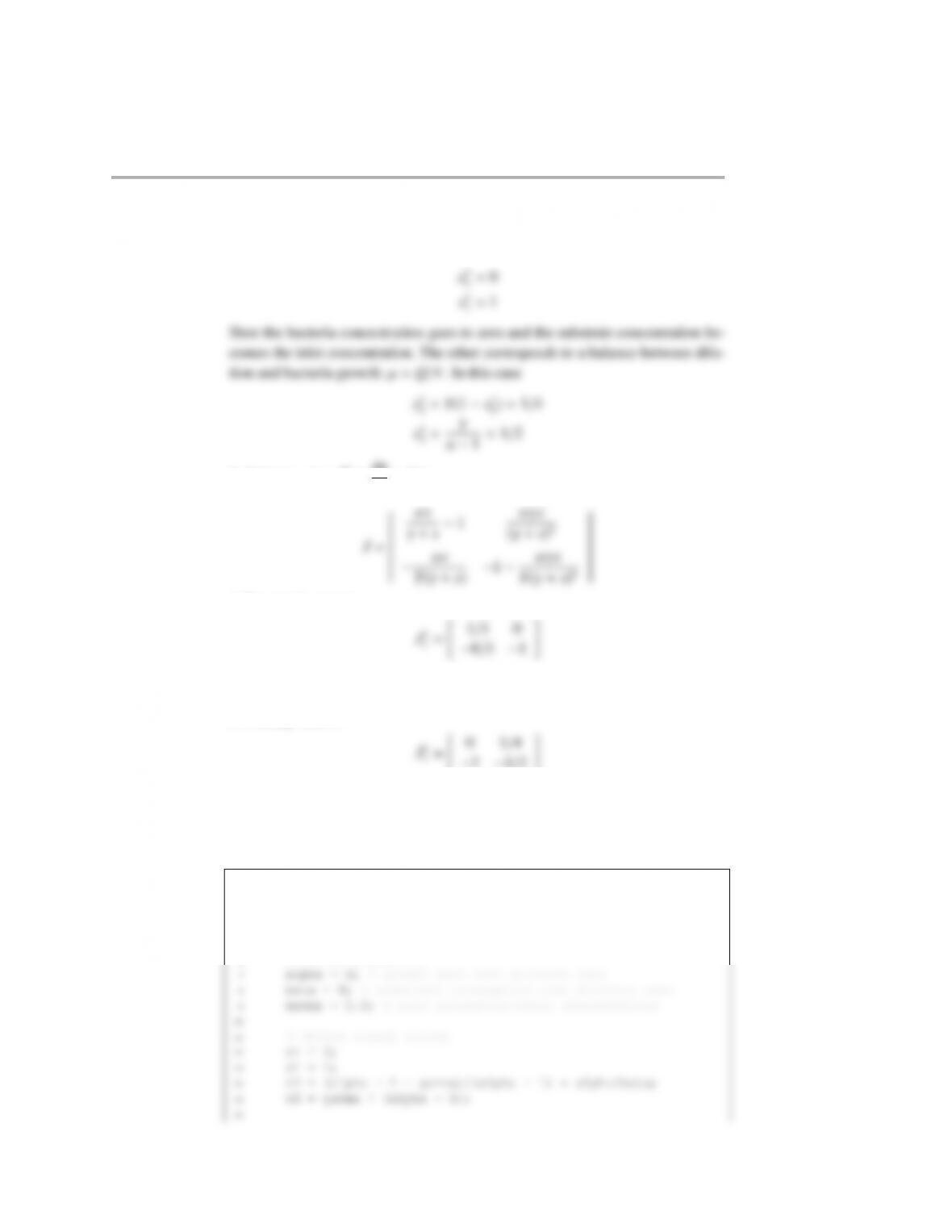
4. For steady state 1:
The eigenvalues of this Jacobian are −1 and 1/3, which makes this fixed point
an unstable saddle point.
For steady state 2:
The eigenvalues of this Jacobian are −1/2 and −1, which makes this point a
stable node.
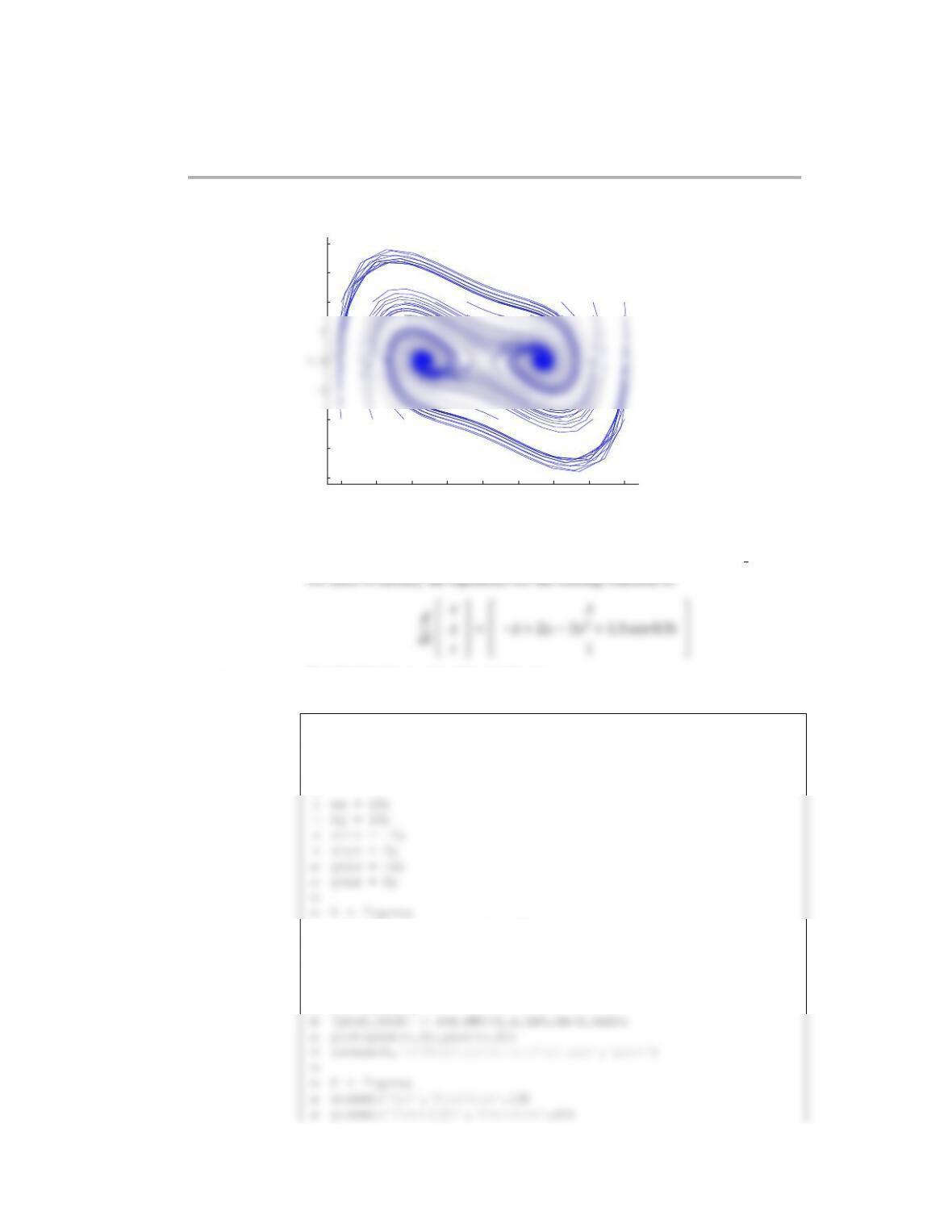
(b) The Matlab solution is:
1function s13c9p123b()
2
3global alpha beta gamma
4close all;
5
6% define parameters
17 % get vector field
18 [x,s] = meshgrid(linspace(0, 1),linspace(0, 1));
19 RHS = zeros(length(x), length(x), 2);
20 for i = 1:length(x)
21 for j = 1:length(x)
32 y2 = RK4([0.1, 0.3], h, Nt);
33
34 %*** make plot ***
35 figure;
36 set(0,‘defaulttextinterpreter’,‘latex’)
47
48 % plot slope field
49 h = streamslice(x, s, RHS(:, :, 1), RHS(:, :, 2));
50 set(h, ‘color’,‘k’);
51 hold off
61
62 end
63
64 function out = f(y)
65