Initial value problems 271
of equations is
dt =k5E
with A(0) =0.75, B(0) =1 and C(0)=D(0)=E(0)=F(0) =0.
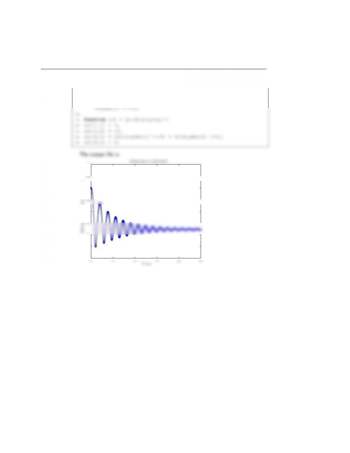
The Matlab file for solving this problem with RK4 is:
1function s14c9p3
2clc
3close all
4set(0,‘defaulttextinterpreter’,‘latex’)
5
6%reaction rates
7krate = [2,1,5,3,1];
8%initial conditions
9x = [0.75;1;0;0;0;0];
10 %parameters for the integration
21 tout = linspace(0,tmax,npts+1);
22
23 Aout(1) = x(1);
24 Bout(1) = x(2);
25 Cout(1) = x(3);
272 Initial value problems
36 k4 = feval(x+h*k3,krate);
37 x=x+h/6*(k1+2*k2+2*k3+k4);
38 %store the output
39 Aout(i) = x(1);
50 ylabel(‘Concentration’,‘FontSize’,14)
51 legend(‘A’,‘B’,‘C’,‘D’,‘E’,‘F’,‘Location’,‘NorthEast’)
52 saveas(g,‘s14c9p3 solution figure.eps’,‘psc2’)
53
54
65 r3 = k(3)*B*C;
66 r4 = k(4)*D*E;
67 r5 = k(5)*E;
68
69 out(1) = -r1 + r2; %A reactions
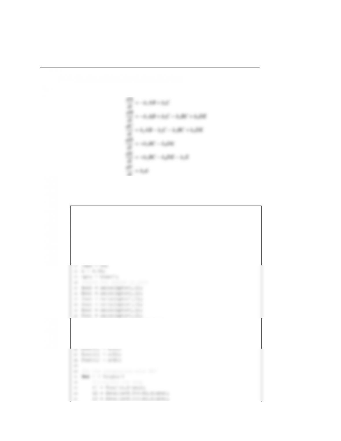
0 1 2 3 4 5 6 7 8 9 10
0
0.1
0.2
0.3
0.4
0.5
0.6
0.7
0.8
0.9
1
Time
Concentration
A
B
C
D
E
F
(4.42) The files for this problem are contained in the folder s12c8p3 matlab.
Define y1=rand y2=r′. Then the residual is
R=“yi+1
1−yi
1−hyi+1
2
yi+1
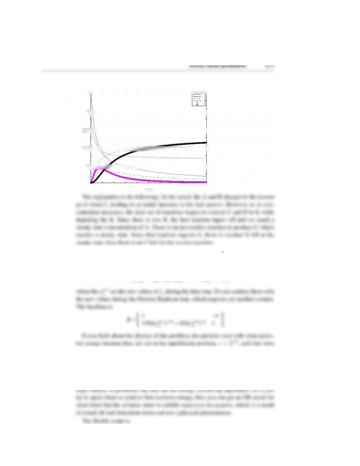
no kinetic energy. However, after integrating for some time, the system appears to
settle into the potential energy minimum and lose its kinetic energy. This is physi-
5
6%initial values and time stepping
7yold = [1.3;0];
8time = 0;
9tmax = 25
20 for i = 1:nsteps
21 ynew = yold; %initial guess
22 R = residual(ynew,yold,h);
23 tol = 1e-5;
24 count = 1;
%8.6f!\n’,time)
32 R = 0;
33 end
34 count = count + 1;
35 end
Initial value problems 275
55 function out = residual(ynew,yold,h)
56 out(1,1) = ynew(1) – yold(1) -h*ynew(2);
57 out(2,1) = ynew(2) – yold(2) -h*(12*ynew(1)ˆ(-13) – …

(5.1) The Jacobian for this system is
J=“πcos(πx1) cos(πx2)−4−πsin(πx1) sin(πx2)+2x2
x2/x1ln x1#
(5.2) We first rewrite the problem as
d
dt “x
˙x#=“˙x
−˙x+2x−3x3#
The steady states correspond to ˙x=0, which makes sense since this is the velocity.
From the second equation, we then require
(5.3) The steady state solution is for cos x=cos y=0, which is all of the possibly combi-
nations of π/2. The Jacobian is
(5.4) From the second equation, the steady states correspond to y1=y2. Substituting into
the first equation gives y2
1−3y2
1+2=y2
1−1=0. So the steady states are (1,1) and
(−1,−1).
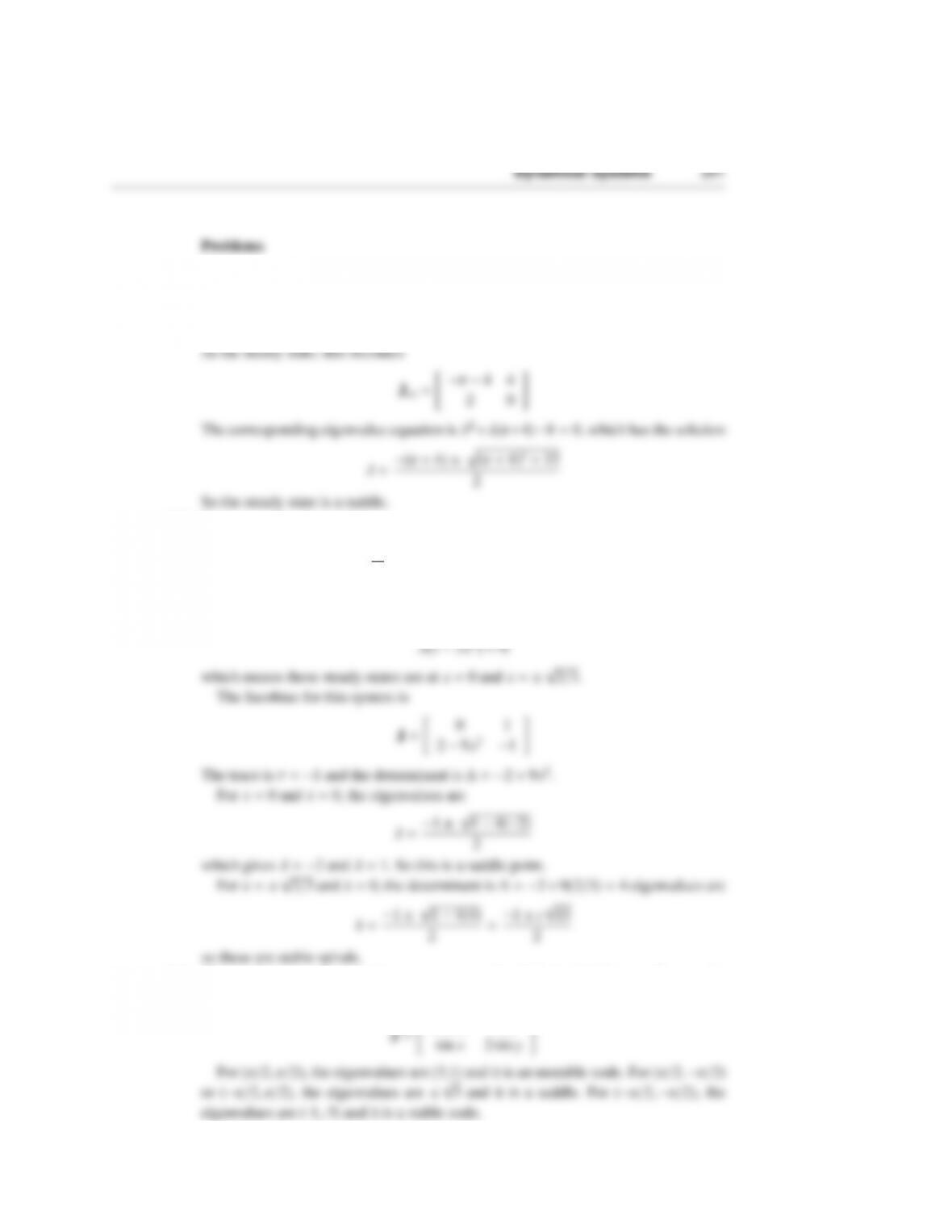
(5.5) The steady states are (−2,−2) and (2,−2). The Jacobian is
J=“2xex2−y2−2yex2−y2
2xy−1−(x/y)2#
Dynamical systems 293
(5.6) Convert this to a system of equations with y1=xand y2=x′:
y′
1=y2
y′
2.
294 Dynamical systems
For the steady state at (-1,0), the Jacobian becomes
(5.8) The steady state Jacobian for this (linear) system is
221
(5.9) The Jacobian is
J=“1+y2y1
3y2
1−1#
(5.10) The steady state equations you need to solve are
3x−2y=0
−3x+2y=0
The solution is y=(3/2)x. Anything on this line is a steady state.
(5.11) (a) From the first equation there are two possible steady states at either y1=−1 or
y2=0 plugging those values into equation 2 we find the steady states are (0,0)
and (−1,−3)
(b) To find eigenvalues fist we must calculate the Jacobian
(5.12) Case 1: The steady states equations are
x1=−x2
and
x2
2+x2=x2(x2+1) =0
Case 2: The steady state equations are
x1=x2
and
x2
2+x2=x2(x2+1) =0
(5.13) The steady state equations are
ax1+bx2=0
bx1+ax2−0
The only solution is (0,0). We need to compute the eigenvalues of
(5.14) a>0
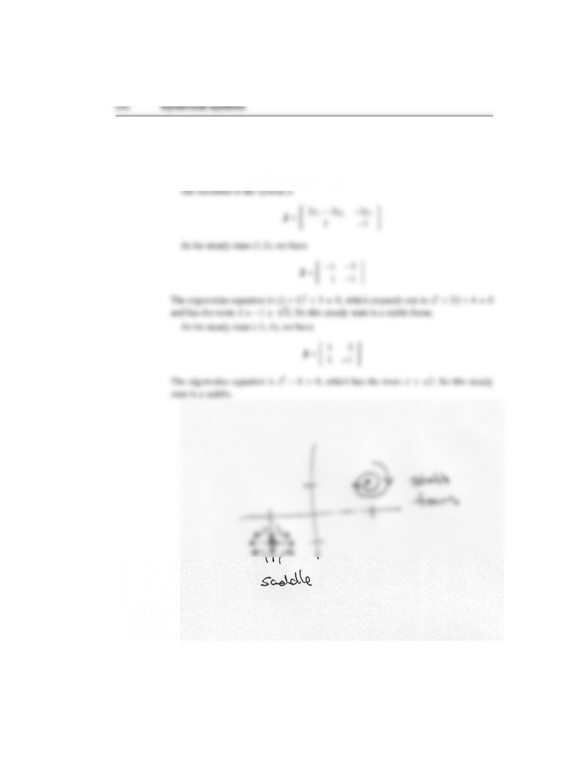
(5.16) The steady states are the solutions to
x(y+x)=0
y(x2−1) =0
From the second equation y=0 or x=±1. For the first equation, x=0 or x=−y. So
there are steady states at (0,0), (1,-1) and (-1,1). The Jacobian for linear stability is
Jss =“−1−1
−2 0 #
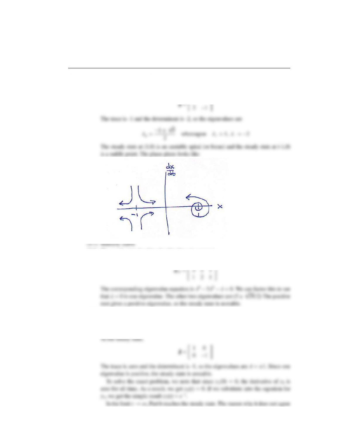
The trace is -1 and the determinant is -2 so
λ=−1±3
2
(5.17) Re(λ)>0, Im(λ)=0
(5.18) (a) f1=v,x(0) =x0,f2=−kx −ξv,v(0) =v0
(b) x=0, v=0
(c) stable
(d) This is a linear problem so A=J:
J=“0 1
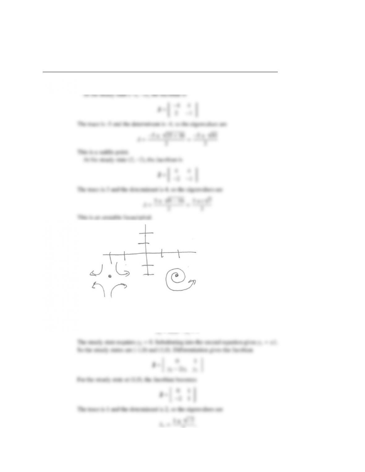
(5.19) The files for this problem are contained in the folder s12c9p2 matlab.
The steady-state equations are
0=2x1−x1x2
0=2x2
1−x2
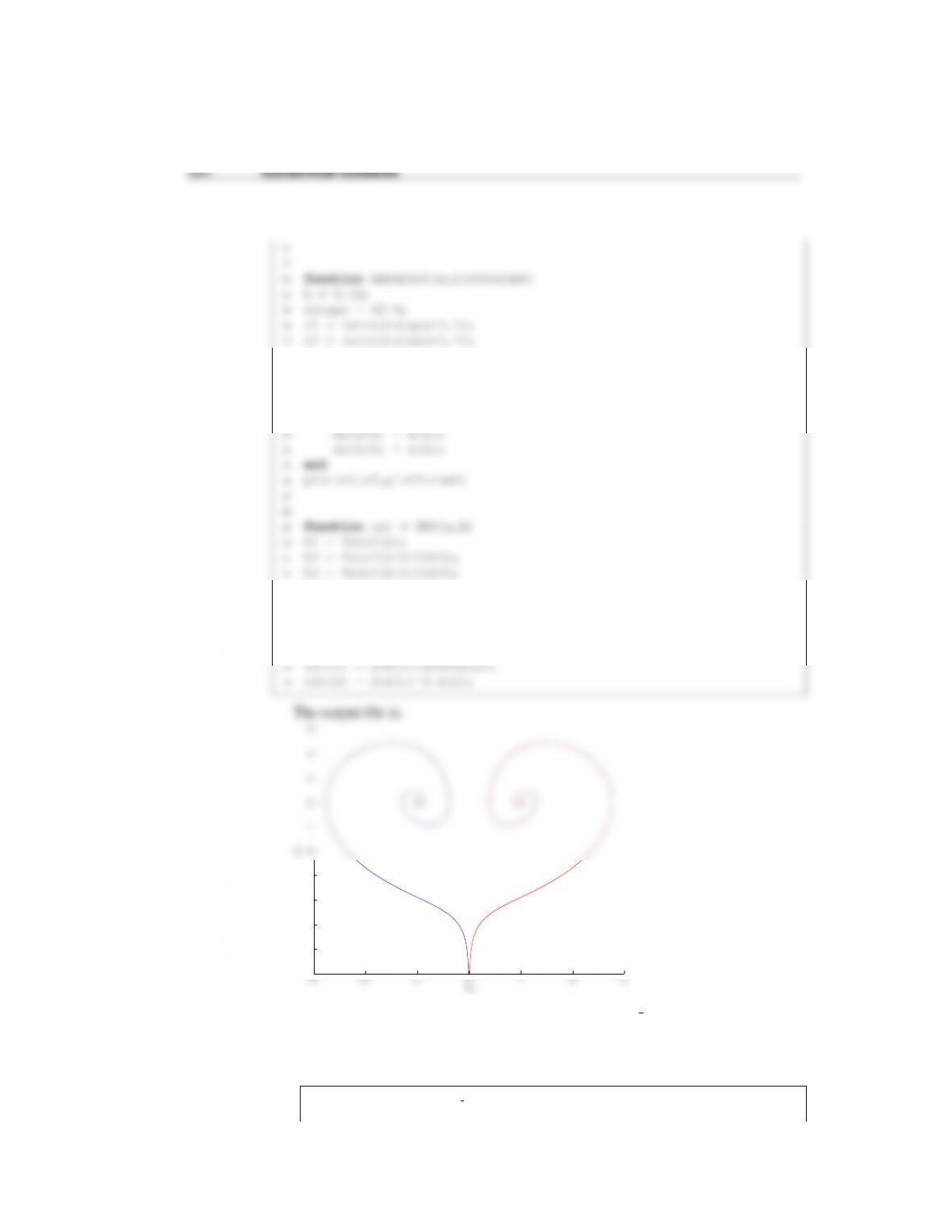
λ=−1±√−15
2
so this is a stable spiral. For the second root, we have
J=“0 1
−4−1#
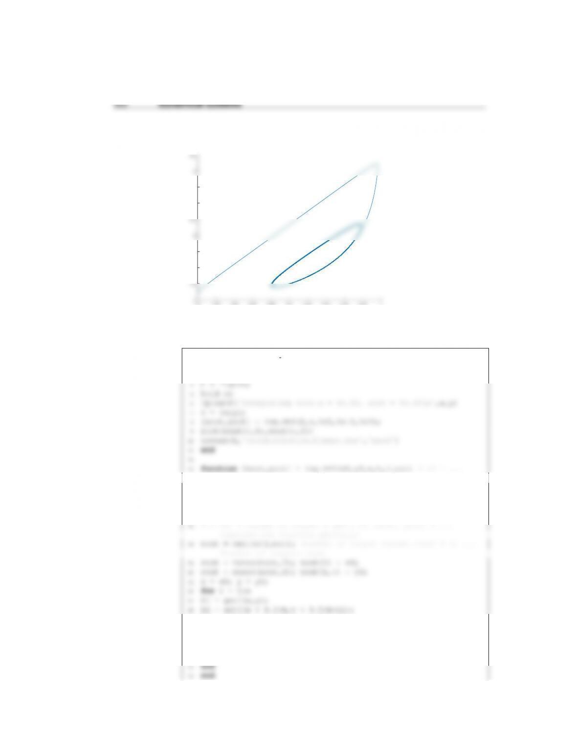
looks like a heart, so I imagine many of your answers to the last question will be no!
The Matlab script is:
1function s12c9p2
2clc
3close all
14
15 hold off
16
17 xlabel(‘$x 1$’,‘FontSize’,14)
18 ylabel(‘$x 2$’,‘FontSize’,14)
28 x1(1) = x(1);
29 x2(1) = x(2);
30
31 for i = 1:nsteps
32 x = RK4(x,h);
43 k4 = feval(x+h*k3);
44 out = x + h/6*(k1+2*k2+2*k3+k4);
45
46
47 function out = feval(x)
12 end
13
14 function [xout,yout] = ivp RK4(x0,y0,n,h,i out) % x0 = …
initial value for x
15 % y0 = initial value for y
24 for i = 1:n
25 k1 = getf(x,y);
26 k2 = getf(x + 0.5*h,y + 0.5*h*k1);
27 k3 = getf(x + 0.5*h,y + 0.5*h*k2);
28 k4 = getf(x + h, y + h*k3);
39 beta = 3;
40 B=22;
41 out=zeros(2,1);
42 out(1,1) = -x1+D*(1-x1)*exp(x2);
43 out(2,1) = -x2+B*D*(1-x1)*exp(x2)-beta*(x2-0);
0.8 0.82 0.84 0.86 0.88 0.9 0.92 0.94 0.96 0.98 1
4
4.5
5
5.5
6
6.5
7
7.5
8
8.5
(b) The Matlab script for this part is:
1function solution figure2
2x=0.9;
3y=6.25;
initial value for x
14 % y0 = initial value for y
15 % n = number of steps to take
16 % h=stepsize
17 count=0;
26 k3 = getf(x + 0.5*h,y + 0.5*h*k2);
27 k4 = getf(x + h, y + h*k3);
28 y = y + (h/6)*(k1 + 2*k2 + 2*k3 + k4); x = x + h;
29 count = count + 1;
30 yout(count,:) = y;
40 out=zeros(2,1);
41 out(1,1) = -x1+D*(1-x1)*exp(x2);
42 out(2,1) = -x2+B*D*(1-x1)*exp(x2)-beta*(x2-0);
43 end
The output file is:
0.86 0.88 0.9 0.92 0.94 0.96 0.98 1
3.5
4
4.5
5
5.5
6
6.5
7
7.5
8
(c) The Matlab script for this part is:
1function solution figure3
2x=0.95;
3y=2.5;
14 [xout1,yout1] = ivp RK4(0,z,1e5,1e-3,1e2);
15 plot(yout1(:,1),yout1(:,2))
16 saveas(h,‘cpc1c solution figure’,‘psc2’)
17 end
18
%number of outputs used
26 xout = zeros(nout,2); xout(1) = x0;
27 yout = zeros(nout,2); yout(1,:) = y0;
28 x = x0; y = y0;
29 for i = 1:n
40 function out = getf(x,y)
41 x1 = y(1);
42 x2 = y(2);
43 D=0.32;
44 beta = 3;
0.5 0.55 0.6 0.65 0.7 0.75 0.8 0.85 0.9 0.95
0.5
1
1.5
2
2.5
3
3.5
4
4.5
(5.21) The files for this problem are contained in the folder s12c9p3 matlab.