Initial value problems 251
51 function out = feval(x,y)
29 tol = 10ˆ-6; %convergence for Newton’s method
252 Initial value problems
30 for i = 1:n steps
31 y old = y new; %zero order continuation method for …
Newton’s method, do not change guess for y new
40 disp(‘Failed to converge!’)
41 err = -1;
42 end
43 end
44 end
h*sin(pi*x new)*cos(pi*y new)*exp(-(x newˆ2+y newˆ2));
55
56 function out = fder(y new,x new,h)
57 out = -1 – …
h*sin(pi*x new)*exp(-(x newˆ2+y newˆ2))*(pi*sin(pi*y new)+2*y new*cos(pi*y new));
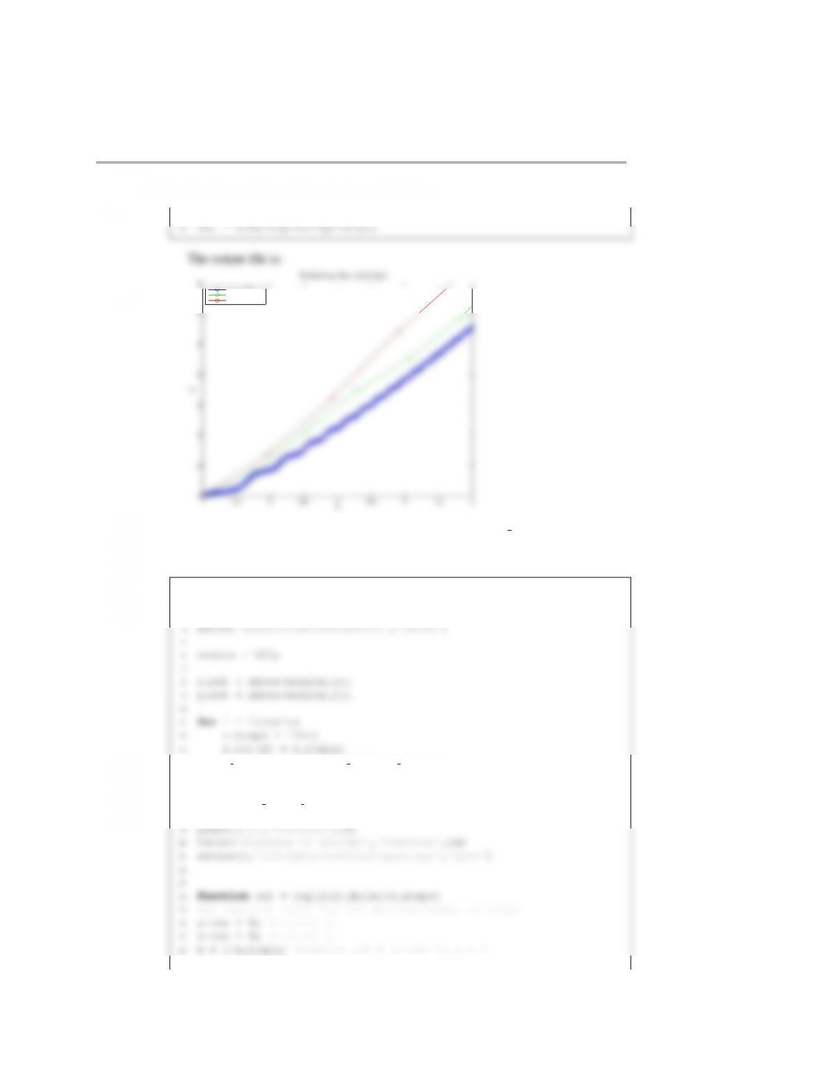
The output file is:
101102103
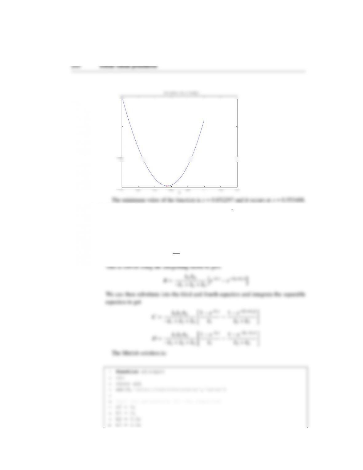
0.34
0.345
0.35
0.355
n
y
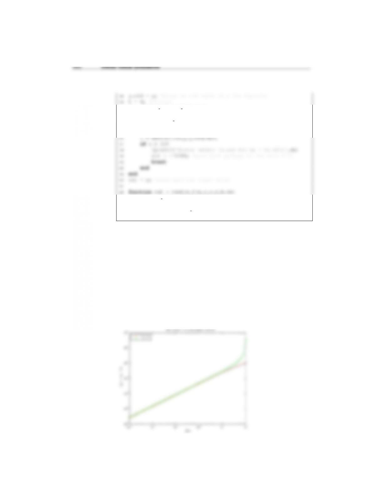
Solut ion to s11c 5p1
(4.37) The files for this problem are contained in the folder s14c8p123 matlab
(a) The Matlab program to solve this problem is:
Initial value problems 253
1function s14c8p1
2close all
3clc
4set(0,‘defaulttextinterpreter’,‘latex’)
15 n = (xmax-xmin)/dx + 1; %total number of steps
16
17 %make the exact solution
18 xplot = linspace(0,xmax,n);
19 y exact = exp(1-cos(xplot));
29 h = figure;
30 plot(xplot,y exact,‘-ok’,xplot,y euler,‘-xr’,…
31 xplot,y RK4,‘-+b’)
32 xlabel(‘$x$’,‘FontSize’,14)
33 ylabel(‘$y$’,‘FontSize’,14)
44 y out = zeros(n,1);
45 y out(1) = y;
46 for j = 2:n
47 y=y+dx*feval(x,y);
48 x=x+dx;
58 for j = 2:n
59 k1 = feval(x,y);
60 k2 = feval(x+dx/2,y+k1*dx/2);
61 k3 = feval(x+dx/2,y+k2*dx/2);
62 k4 = feval(x+dx,y+k3*dx);
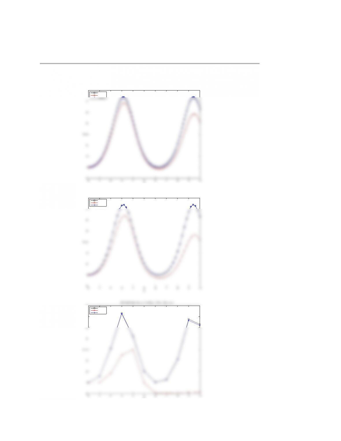
produced by the program are:
0 1 2 3 4 5 6 7 8 9 10
0
1
2
3
4
5
6
7
8
x
y
Solut ion t o s 14c 8p1 f or ∆x=0.001
E x ac t
E u l e r
R K 4
0 1 2 3 4 5 6 7 8 9 10
0
1
2
3
4
5
6
7
8
x
y
Solut ion t o s 14c 8p1 f or ∆x=0.01
E x ac t
E u l e r
R K 4
Initial value problems 255
0 1 2 3 4 5 6 7 8 9 10
0
1
2
3
4
5
6
7
8
x
y
Solut ion t o s 14c 8p1 f or ∆x=0.1
E x ac t
E u l e r
R K 4
0 1 2 3 4 5 6 7 8 9 10
0
1
2
3
4
5
6
7
8
x
y
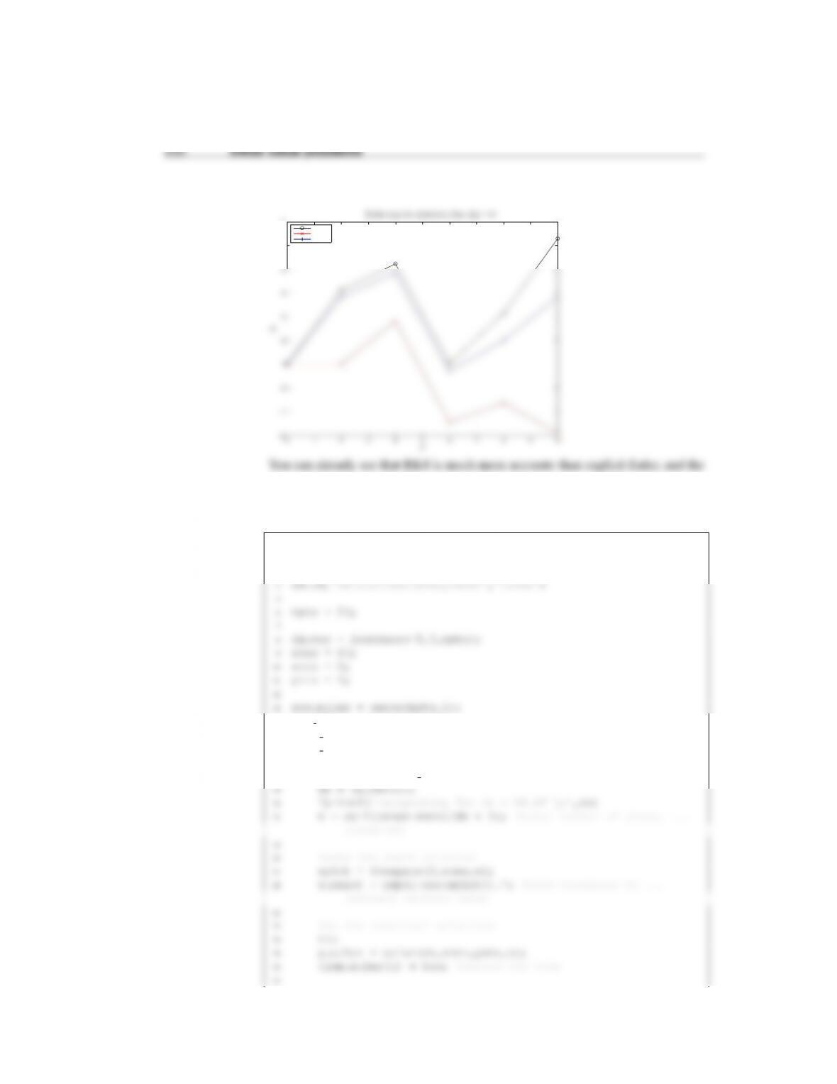
Solut ion t o s 14c 8p1 f or ∆x=0.2
E x ac t
E u l e r
R K 4
0 1 2 3 4 5 6 7 8 9 10
0
1
2
3
4
5
6
7
8
x
y
Solut ion t o s 14c 8p1 f or ∆x=1
E x ac t
E u l e r
R K 4
Initial value problems 257
32 tic
33 y RK4 = RK4(dx,xmin,ymin,n);
34 time RK4(i) = toc;
35
46 legend(‘Euler’,‘RK4’,‘Location’,‘NorthWest’)
47 title(‘Solution to s14c8p2: Error’,‘FontSize’,14)
48 saveas(h,‘s14c8p2 solution figure1.eps’,‘psc2’)
49
50 h = figure;
61 y = ymin;
62 y out = zeros(n,1);
63 y out(1) = y;
64 for j = 2:n
65 y=y+dx*feval(x,y);
76 for j = 2:n
77 k1 = feval(x,y);
78 k2 = feval(x+dx/2,y+k1*dx/2);
79 k3 = feval(x+dx/2,y+k2*dx/2);
80 k4 = feval(x+dx,y+k3*dx);
10−5 10−4 10−3 10−2 10−1 100
10−10
10−9
10−8
10−7
10−6
10−5
10−4
10−3
10−2
10−1
100
∆x
||y∗ −y||/n
Solut ion to s14c 8p2: Error
E u l e r
R K 4
10−5 10−4 10−3 10−2 10−1 100
10−5
10−4
10−3
10−2
10−1
100
101
∆x
Solut ion time ( se conds )
So lut ion t o s 14 c 8p 2: T i me
E u l e r
R K 4
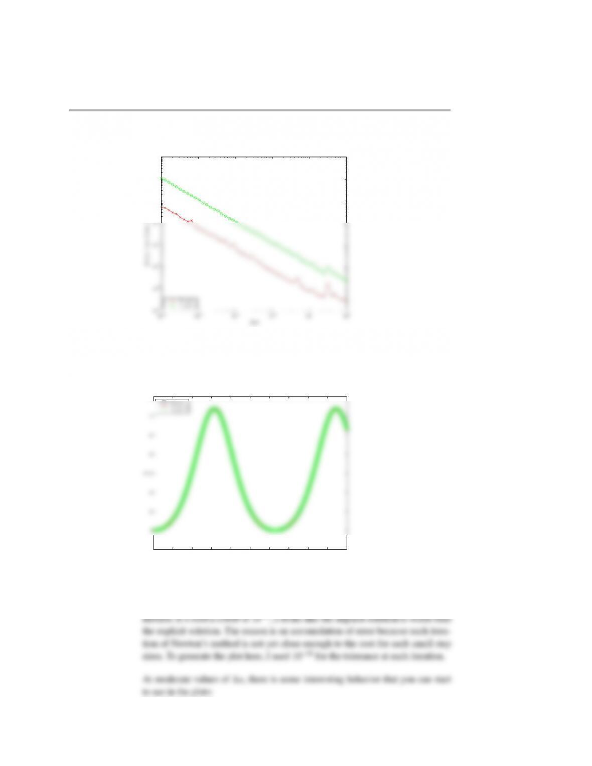
Accuracy: The improved accuracy of RK4 is evident from this figure at given
values of ∆x. It is interesting that the accuracy fluctuates so much with the par-
ticular value of ∆x. Remember that the truncation error depends not only on the
value of ∆x, but also on the smoothness of the function. So as we change ∆x,
we evaluate the slopes at different points. If the function changes quickly, then
Initial value problems 259
explicit Euler. There are 4 function evaluations in RK4 compared to 1 function
evaluation in explicit Euler, but you should not expect a ratio of exactly 4 —
there are still a few more calculations besides just evaluating the function. The
noise at the small values of ∆xare just system noise from the computer doing
5
6npts = 50;
7dx vec = logspace(-5,0,npts);
8xmax = 10;
9xmin = 0;
20 fprintf(‘Integrating for dx = %8.6f \n’,dx)
21 n = ceil((xmax-xmin)/dx + 1); %total number of steps, …
round-off
22
23 %make the exact solution
33 y implicit = implicit euler(dx,xmin,ymin,n);
34 time implicit(i) = toc;
35
36 if i == 1
37 h = figure;
47 saveas(h,‘s14c8p3 solution figure1.eps’,‘psc2’)
48 end
49
50 if i == 25
51 %good example to see the issue at modest dx
62 saveas(h,‘s14c8p3 solution figure2.eps’,‘psc2’)
63 end
64
65 if i == 44
66 %this is a good example to see the problem for …
76 ‘Location’,‘NorthWest’)
77 saveas(h,‘s14c8p3 solution figure3.eps’,‘psc2’)
78 end
79
80 %compute the error in the solution
Initial value problems 261
93
94 h = figure;
95 loglog(dx vec,time euler,‘-xr’,dx vec,time implicit,‘-og’)
96 xlabel(‘$\Delta x$’,‘FontSize’,14)
107 y out(1) = y;
108 for j = 2:n
109 y=y+dx*feval(x,y);
110 x=x+dx;
111 y out(j) = y;
122 k2 = feval(x+dx/2,y+k1*dx/2);
123 k3 = feval(x+dx/2,y+k2*dx/2);
124 k4 = feval(x+dx,y+k3*dx);
125 y = y + dx/6*(k1 + 2*k2 + 2*k3 + k4);
126 x=x+dx;
137 y out = zeros(n,1);
138 y out(1) = y;
139 for j = 2:n
140 %Newton’s method solution using old value as guess
141 x=x+dx;%use the new value of x here!
151 f = newton f(x,y,y old,dx);
152 while abs(f) >1e-10
153 df = newton df(x,dx);
154 y = y – f/df; %Newton’s method update
155 k=k+1;
166 out = y – y old – dx*feval(x,y);
167
168 function out = newton df(x,dx)
169 out = 1 – dx*sin(x);
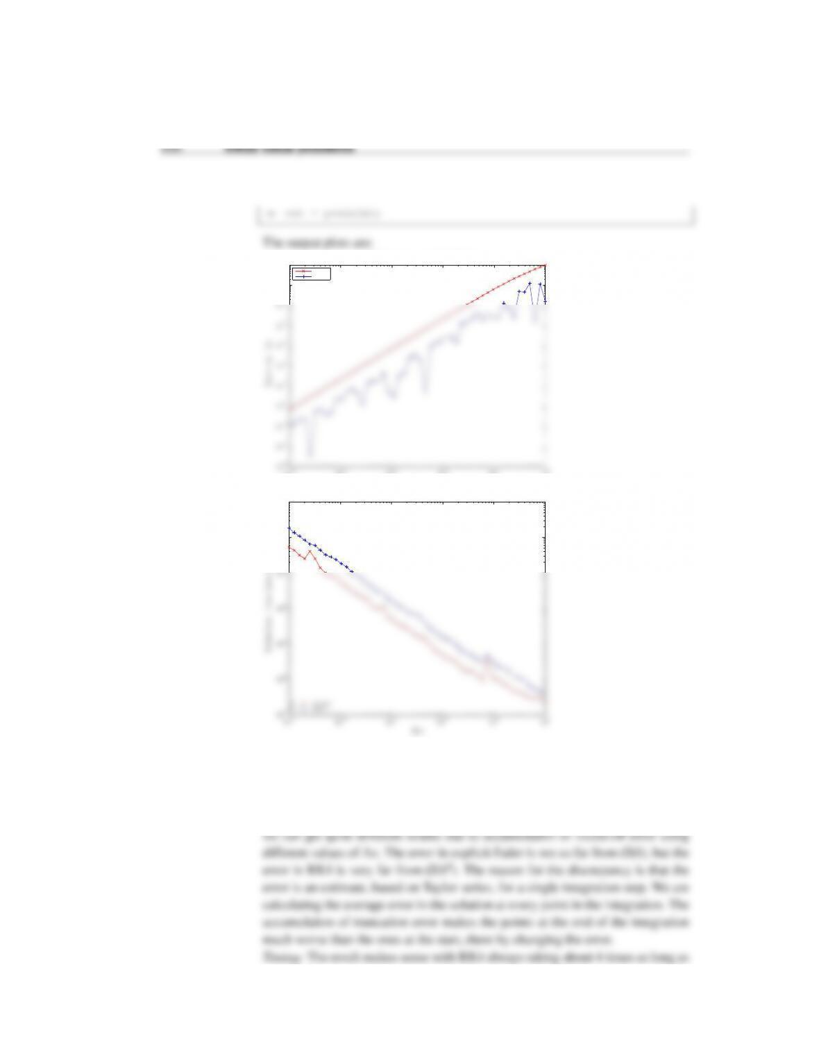
The required output is:
10−5 10−4 10−3 10−2 10−1 100
10−8
10−6
10−4
10−2
100
102
104
∆x
||y∗ −y||/n
Solut ion to s14c 8p3: Err or
E x p l i c i t
I m p l i c i t
Initial value problems 263
10−5 10−4 10−3 10−2 10−1 100
10−5
10−4
10−3
10−2
10−1
100
101
102
∆x
Solut ion time ( se conds )
So lut ion t o s 14 c 8p 3: T i me
E x p l i c i t
I m p l i c i t
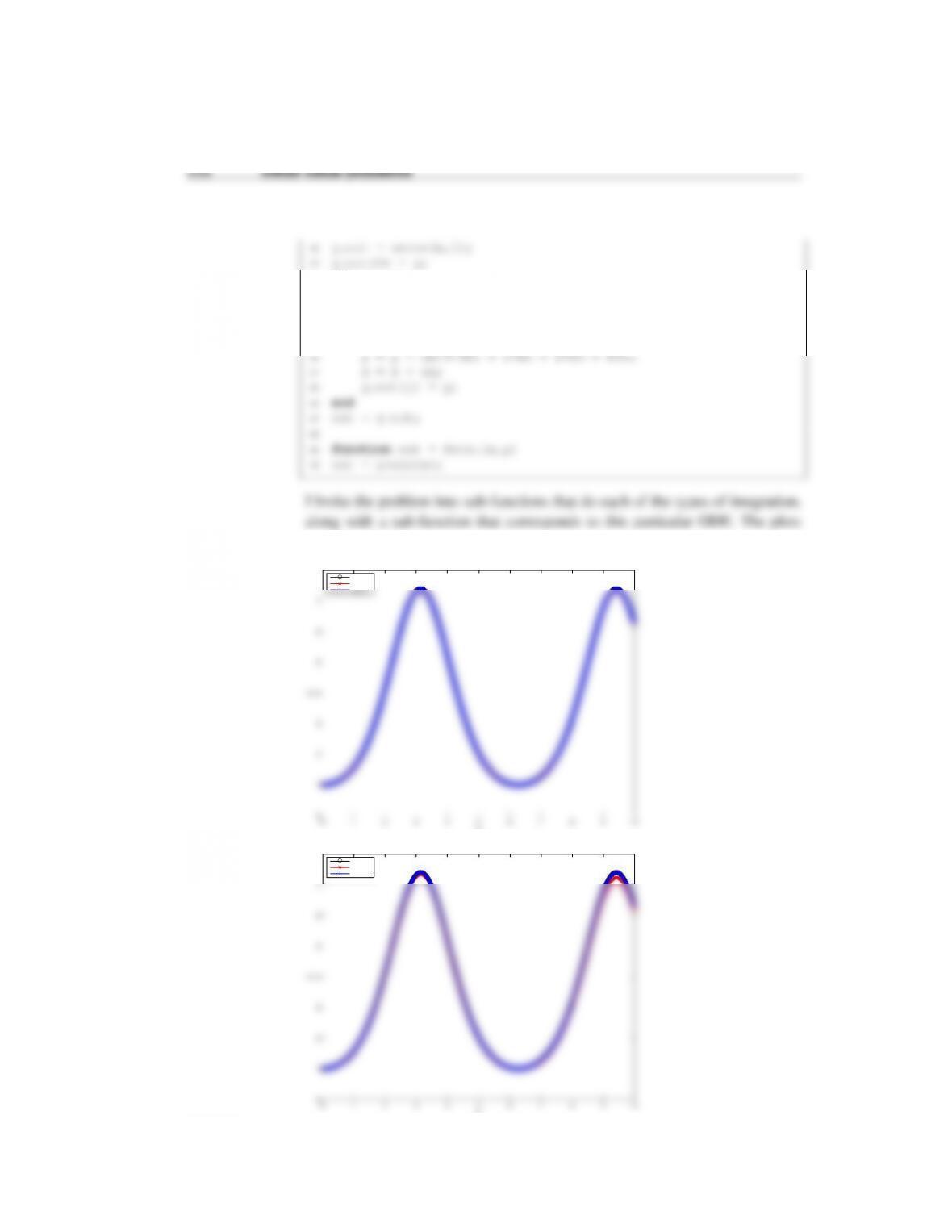
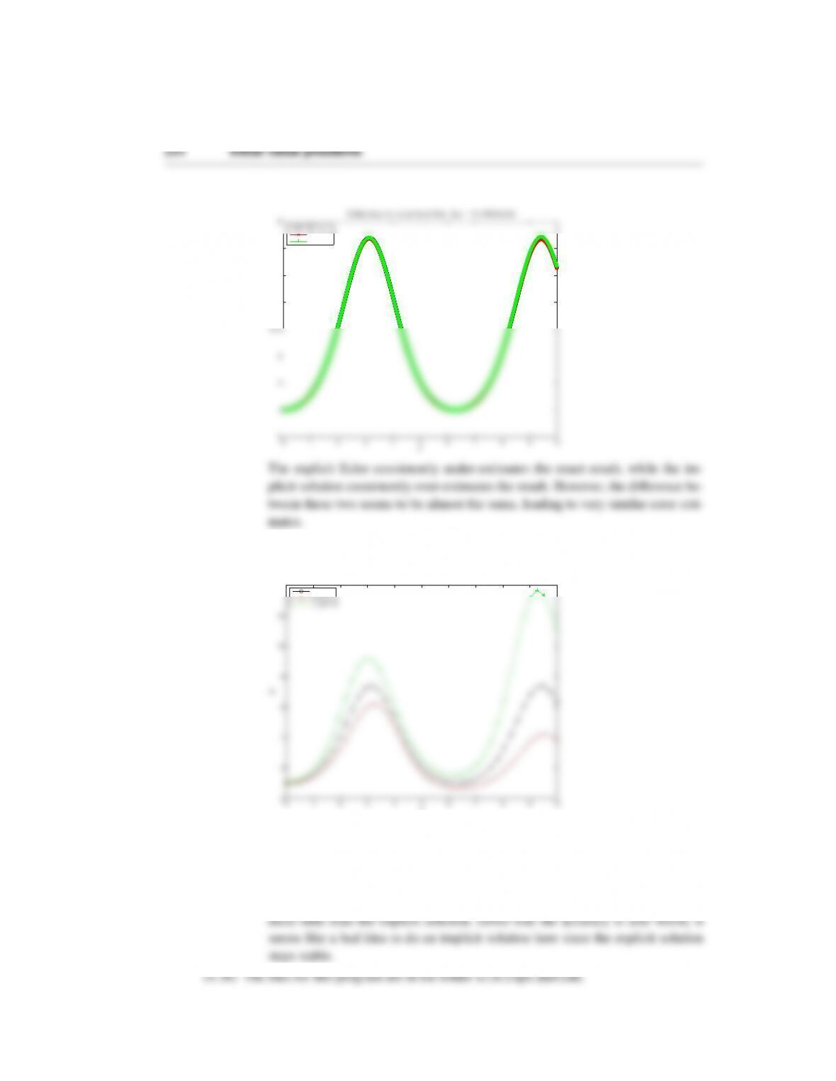
Accuracy: To understand the accuracy, it is useful to look at some representative
plots corresponding to the three different types of behavior. At very small step
sizes, the solutions look almost identical:
0 1 2 3 4 5 6 7 8 9 10
0
1
2
3
4
5
6
7
8
x
y
Solut ion t o s 14c 8p3 f or ∆x=1e –05
E x ac t
E x p l i c i t
I m p l i c i t
The error is also very small. In either case, it makes no difference in the plots and
you could only tell them apart by subtracting the solutions. Note that the results
Initial value problems 265
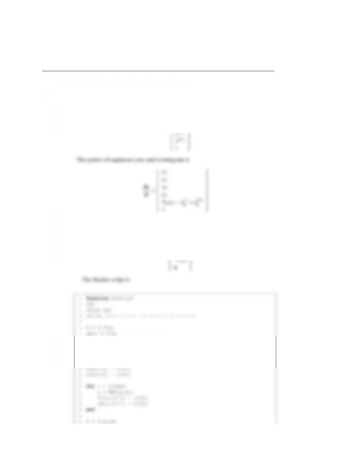
To convert this high-order, non-autonomous IVP to a system of autonomous equa-
tions, define the vector
y=
y
y′
y′′
1
with the initial conditions
y=
−1
1/2
−1/3
1/4
8y = [-1;1/2;-1/3;1/4;-1/5;0];
9
10 y2out = zeros(npts+1,1);
11 y4out = zeros(npts+1,1);
12
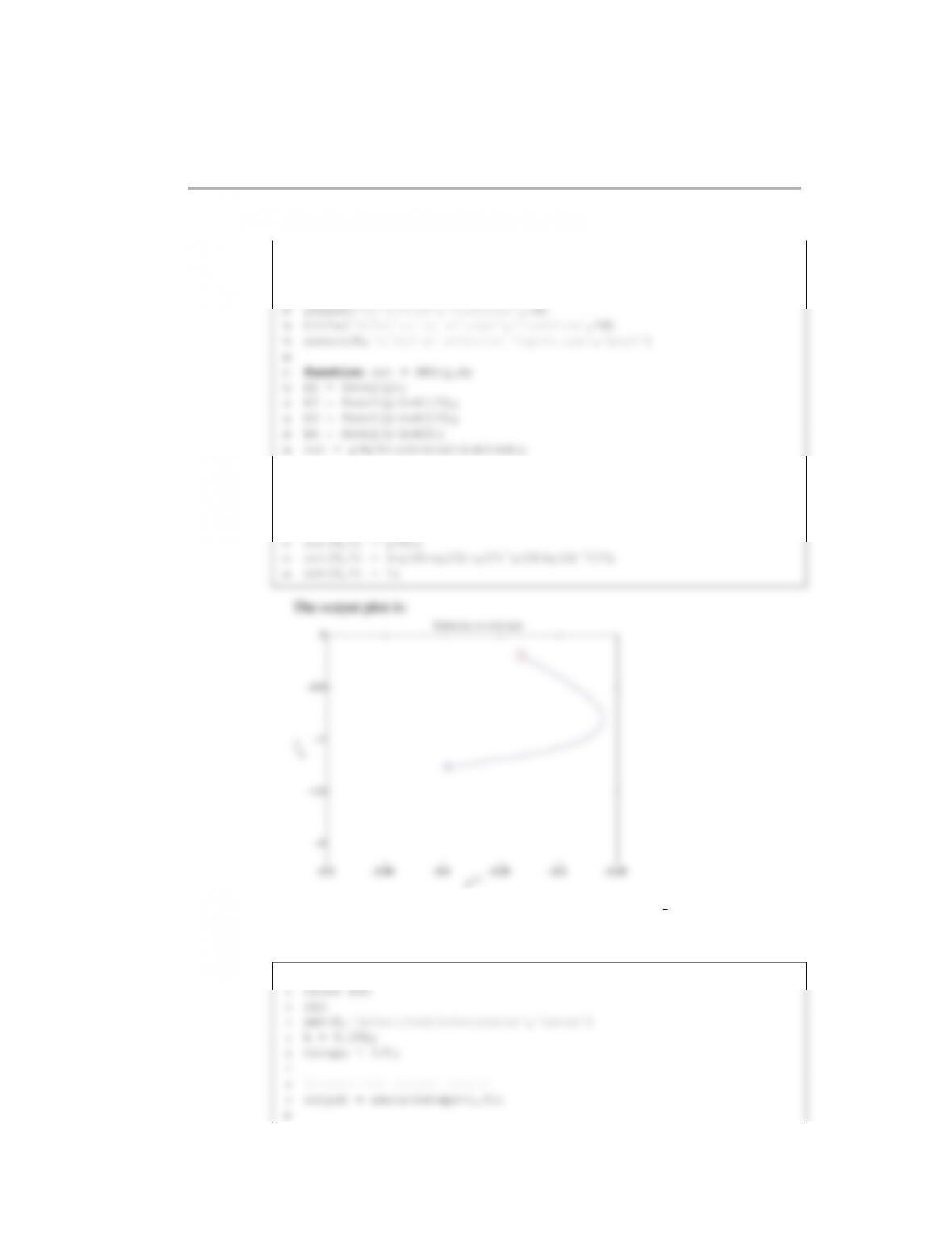
266 Initial value problems
23 plot(y2out,y4out,‘-‘,y2out(1),y4out(1),‘or’,y2out(npts),…
24 y4out(npts),‘bx’,‘MarkerSize’,14);
25 axis([-0.5,-0.25,-2.2,0])
26 xlabel(‘$yˆ{(2)}$’,‘FontSize’,14)
37
38 function out = feval(y)
39 out(1,1) = y(2);
40 out(2,1) = y(3);
41 out(3,1) = y(4);
1function s11c6p1
Initial value problems 267
11 %initial conditions
12 y = [1, -0.5, 0.7, 0];
13 output(1,:) = y;
14
25 yp left = output(i,2);
26 yp right = output(i+1,2);
27 end
28 end
29
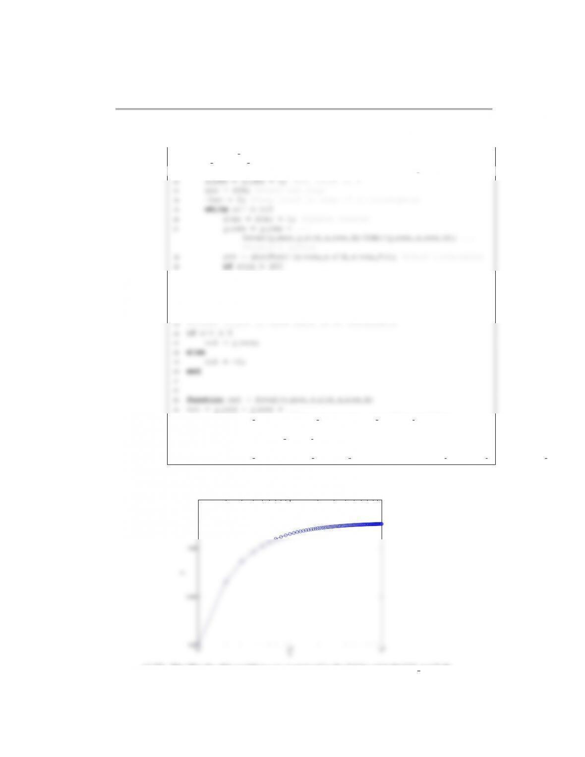
occurs at x = %8.6f.\n’,y min,x min)
37
38
39 h = figure;
40 plot(output(:,4),output(:,1),‘-b’,x min,y min,‘or’,‘MarkerSize’,8)
51 k4 = feval(y+h*k3);
52 out = y + (h/6)*(k1 + 2*k3 + 2*k3 + k4);
53
54 function out = feval(y)
55 out(1) = y(2);
Initial value problems 269
11
12 %set up the time step parameters
13 dt = 0.1;
14 tmax = 10;
25 Ce = zeros(npts,1);
26 D = zeros(npts,1);
27 De = zeros(npts,1);
28
29 A(1) = A0; Ae(1) = A0;
40 D(i) = y(4);
41 Ae(i) = ye(1);
42 Be(i) = ye(2);
43 Ce(i) = ye(3);
44 De(i) = ye(4);
55 ylabel(‘Concentration’,‘FontSize’,14)
56 title(‘Solution to s13c8p23’,‘FontSize’,14)
57 saveas(h,‘s13c8p23 solution figure.eps’,‘psc2’)
58
59
270 Initial value problems
70 function out = getf(y,k1,k2,k3)
71 %unpack the y vector for convenience
72 A = y(1);
73 B = y(2);
84 B = k1*A0/(-k1+k2+k3)*(exp(-k1*t)-exp(-(k2+k3)*t));
85 C = k1*k2*A0/(-k1+k2+k3)*((exp(-(k2+k3)*t)-1)/(k2+k3) + …
(1-exp(-k1*t))/k1);
86 D=C*k3/k2;
87 out = [A,B,C,D];
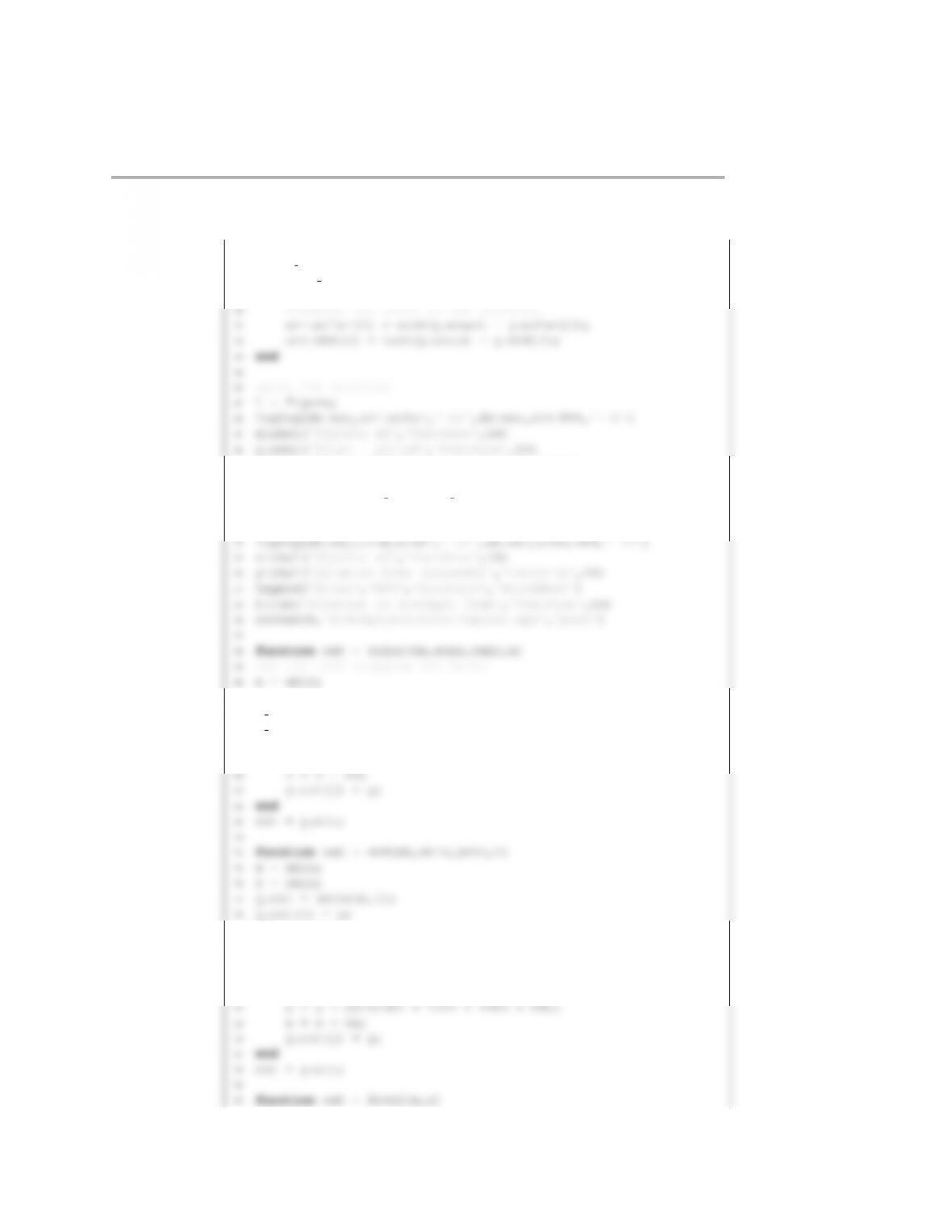
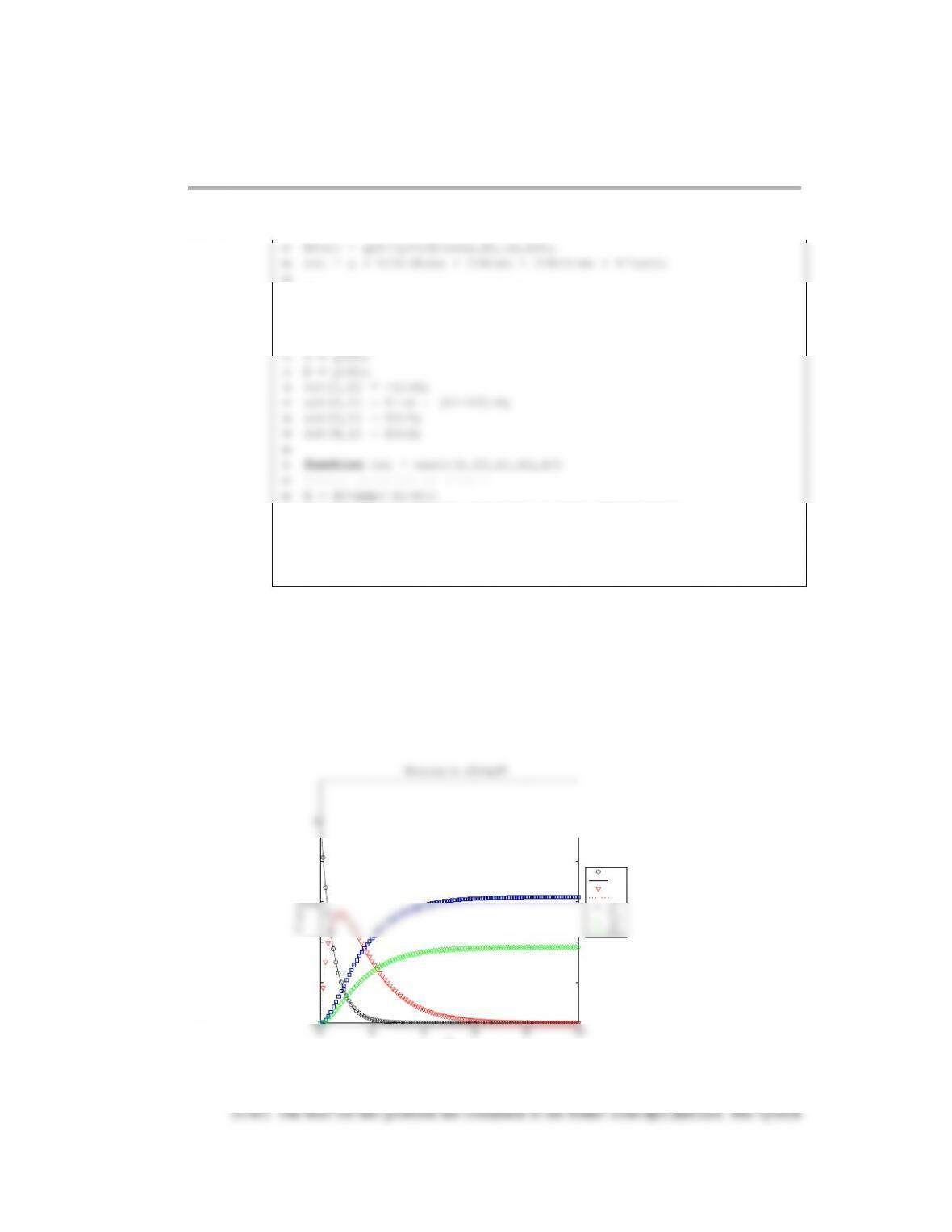
The comparison of the numerical and exact solutions is:
0 2 4 6 8 10
0
0.2
0.4
0.6
0.8
1
t
C on ce nt ra ti on
Solut ion to s 13c 8p23
A
Ae
B
Be
C
Ce
D
De