Initial value problems 231
For the third equation, let y3=xso we get
d
y0
y1
y1
y2
y0
y1
1
0
1/y0#,“y0
(4.20) First expand the term (x2y)′′:
to get the differential equation
Define the vectors
y
x
y2
−4y3y2−y1(1 +cos y3)
1+y2
3
1
3
0
The system of autonomous ODEs is
dx
(4.21) Define y0=y,y1=y′and y2=xso that we get
y0
y2
y1
1
For implicit Euler, we have yi+1−hf(yi+1)−yi=0. The residual vector is then
yi+1
0−hyi+1
1−yi
0
yi+1
2−h−yi
2
232 Initial value problems
The elements of the Jacobian are Ji j =∂Ri/∂yi+1
j:
1−h0
0 0 0
(4.22) If the vector below was used
x
t
then the update scheme can be written as
where
1
The Jacobian for this nonlinear system of equations is
100
001
0 1 0
0 0 0
If you prefer to write it terms of the entries in zthen you get
100
001
0 1 0
0 0 0
(4.23) dy/dt =sin ycos y1/2,y(0) =1 solved by RK4
(4.24) You should first do the normal change of variables:
which gives the system of ODEs:
dt
Initial value problems 233
dt
We want to solve these using implicit Euler, which gives
Rewrite the equations as residuals
The initial guess for the Newton-Raphson on the first step is
which gives an initial residual vector of
−1
001
(4.25) The linear stability condition requires the solution of the linear problem
dy
dt
=−λy
We then need to apply the midpoint formula with f(xi,yi)=−λyi,
h≤2/λ
(4.26) The linear stability equation is
dy
dt
=−λy
Apply the method
(4.27) For linear stability, we consider f(x,y)=−λy. For this problem, k1=−λyiso
k2=−λ yi+3
4k1h!=−λyi+3
4λ2yih
(4.28) To determine stability, we need to analyze
dy
dt
=f(y)=−λy
This means that
66−3hλ+(hλ)2
236 Initial value problems
(4.29) (a) Implicit Euler
(b) The equations are
dy1
=y2
1+y1y2
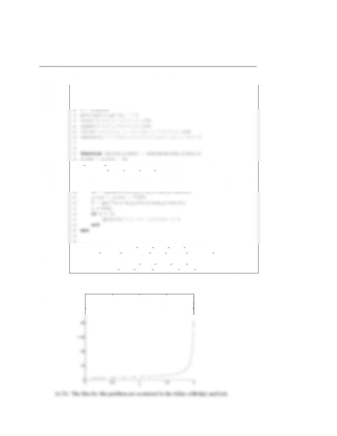
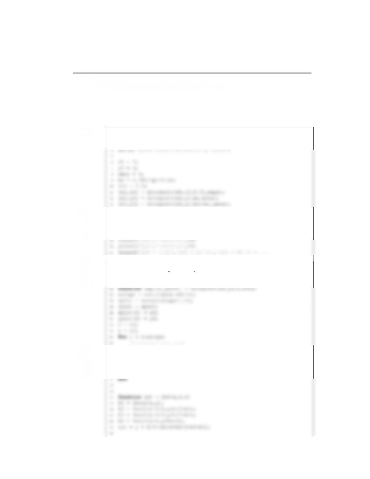
(4.30) The files for this problem are in the folder s13c8p1 matlab.
For implicit Euler, we need to solve
The Matlab script is:
1function s13c8p1
2clc
3close all
4set(0,‘defaulttextinterpreter’,‘latex’)
5
6h = 0.001;
7xmax = 2;
8npts = xmax/h + 1;
9
Initial value problems 237
21 xplot(i) = x;
22 yplot(i) = y;
23 end
24
35 y new = y old; %initial guess, OK for small time steps
36 f = getf(x old,y old,x new,y new,h);
37 k = 0; %counter
38
39 while abs(f) >1e-8
50 function out = getf(x old,y old,x new,y new,h)
51 out = y new – y old – h*(y newˆx new – x new*log(y new));
52
53 function out = getdf(x old,y old,x new,y new,h)
54 out = 1 – h*(x new*y newˆ(x new-1)- x new/y new);
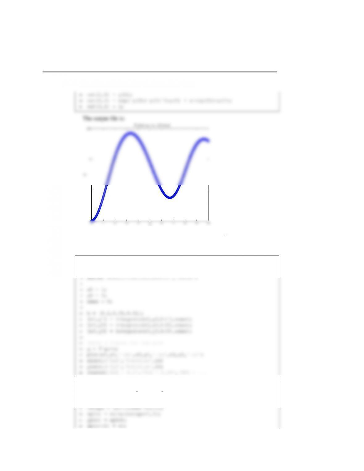
The output file is:
0 0.5 1 1.5 2
0
10
20
30
40
50
60
x
y
S ol ut ion t o s 13c 8p 1
238 Initial value problems
The Matlab script is:
1function s10c6p1
= 0. We can solve this
12 %using RK4 in the vectorized form.
13 close all
14 clc
15 set(0,‘defaulttextinterpreter’,‘latex’)
26 %put in the starting values for y out
27 y out(1,1) = 1;
28 y out(2,1) = 0;
29 y out(3,1) = x start;
30
40 yplot = y out(1,:);
41 h = figure;
42 plot(xplot,yplot,‘:ob’,‘MarkerSize’,8)
43 xlabel(‘$x$’,‘FontSize’,14)
44 ylabel(‘$y$’,‘FontSize’,14)
Initial value problems 239
34 y = rk4(x,y,h);
35 x = x+h;
36 %record the output for plotting
37 xplot(i+1) = x;
38 yplot(i+1) = y;
49 function out = feval(x,y)
50 out = x/sqrt(y)+sin(pi*x*y);
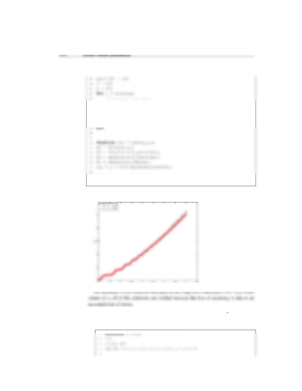
The output file is:
1 1.5 2 2.5 3 3.5 4 4.5 5 5.5
2
3
4
5
6
7
8
x
y
S ol ut io n f or s 12 c 8p 1
h= 0 . 2
h= 0 . 0 8
h= 0 . 0 1
The accuracy of the solution increases as the step size hdecreases. For very small
values of x, all of the solutions are similar because the loss of accuracy is due to an
accumulation of errors.
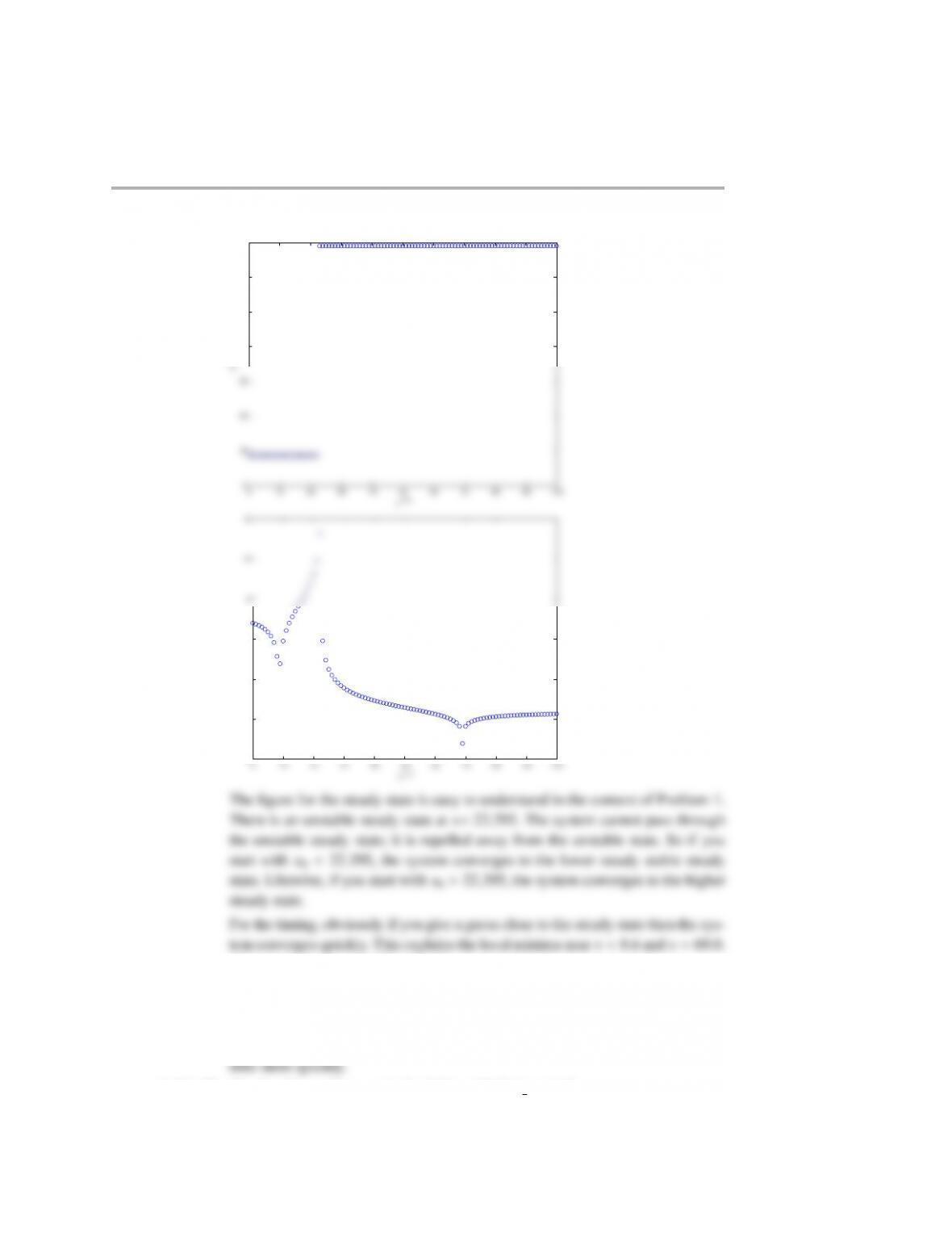
(4.33) (a) The files for this problem are contained in the directory s15c8p1 matlab.
The Matlab file for this problem is
Initial value problems 241
6%problem parameters
7k = [0.0015;0.15;3.5;20];
8
9
20 axis([0,100,-40,40])
21 saveas(g,‘s15h8p1 solution fig.eps’,‘psc2’)
22
23 %compute the roots for good guesses and check stability
24 x = [12,18,72];
35 fprintf(‘\t Stable steady state.\n\n’)
36 end
37
38 function x = get root(x,k)
39 i = 1;
50 end
51 fprintf(‘\t Converged with x = %9.6f with |f(x) |= %6.4e …
\n’,x,abs(f))
52
53 function out = getf(x,k)
Initial value problems 243
for an initial perturbation ∆x0. If κ > 0 the system is unstable, if κ < 0 then the
system is stable.
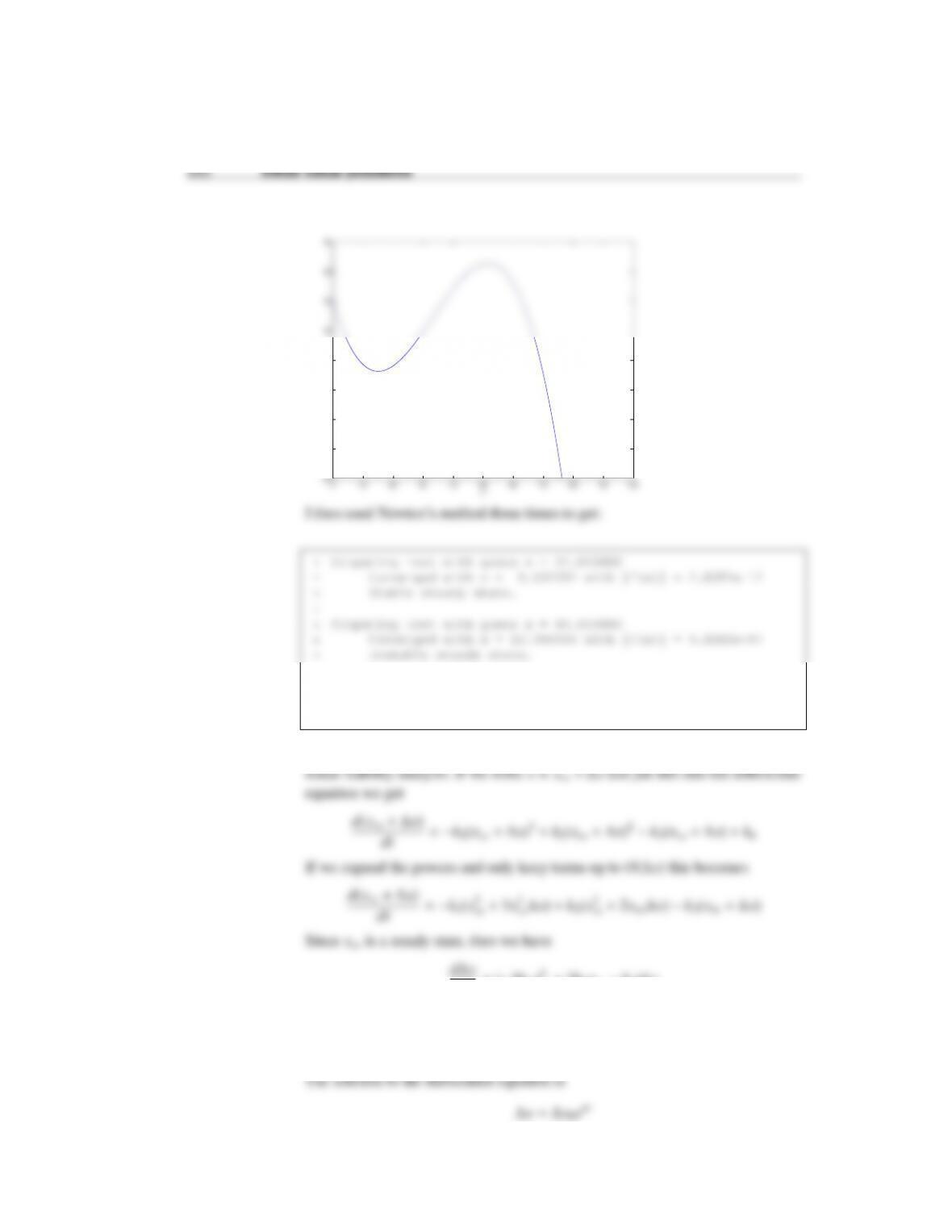
You can also see this result (without the rigorous math) by looking at the function
itself. To be a stable steady state, you need to have f(xss −∆x)>0 and f(xss +
7k = [0.0015;0.15;3.5;20];
8
9%get stable steady states from part 1
10 root1 = get root(12,k);
11 root2 = get root(72,k);
22 x = 0;
23 plot integration(x,k,tmax,root1,root2,‘ob’)
24 x = 15;
25 plot integration(x,k,tmax,root1,root2,‘or’)
26 x = 30;
37 dt = 1e-4;
38 tstep = 1000; %number of steps per plot
39 t = 0;
40 plot(t,x,s)
41 while dx1 >tol && dx2 >tol
51 if t>tmax
52 fprintf(‘Did not reach steady state at t = %8.6f \n’,t)
53 break
54 end
55 end
65 function x = get root(x,k)
66 i = 1;
67 f = getf(x,k);
68 tol = 1e-6;
69 fprintf(‘Computing root with guess x = %8.6f \n’,x)
79
80 function out = getf(x,k)
81 out = -k(1)*xˆ3 + k(2)*xˆ2 – k(3)*x + k(4);
82
83 function out = getdf(x,k)
Initial value problems 245
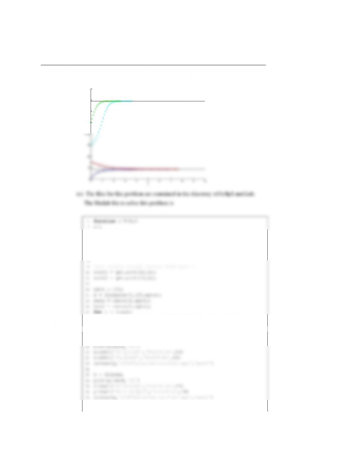
0 1 2 3 4 5 6 7 8 9 10
0
10
20
30
40
50
60
70
80
t
x
(c) The files for this problem are contained in the directory s15c8p3 matlab.
The Matlab file to solve this problem is
1function s15h8p3
2clc
3close all
4set(0,‘defaulttextinterpreter’,‘latex’)
5
6%problem parameters
7k = [0.0015;0.15;3.5;20];
18 [tend(i),xend(i)] = integrate(x(i),k,root1,root2);
19 fprintf(‘x0 = %8.4f \t xss = %8.4f \t t = %8.4f …
\n’,x(i),xend(i),tend(i))
20 end
21 g = figure;
32
33 function [t,x] = integrate(x,k,root1,root2)
246 Initial value problems
34 tmax = 100;
35 dx1 = abs(x – root1);
46 if t>tmax
47 fprintf(‘Did not reach steady state at t = %8.6f \n’,t)
48 break
49 end
50 end
60 function x = get root(x,k)
61 i = 1;
62 f = getf(x,k);
63 tol = 1e-6;
64 fprintf(‘Computing root with guess x = %8.6f \n’,x)
74
75 function out = getf(x,k)
76 out = -k(1)*xˆ3 + k(2)*xˆ2 – k(3)*x + k(4);
77
78 function out = getdf(x,k)
Initial value problems 247
0 10 20 30 40 50 60 70 80 90 100
0
10
20
30
40
50
60
70
x(0 )
xs s
0 10 20 30 40 50 60 70 80 90 100
0
2
4
6
8
10
12
x(0 )
t(xs s)
If you get near the unstable state, the system converges more slowly because you
need to travel the greatest distance to the steady state. The lower times to reach
the upper stable steady state compared to the lower steady state are explained by
looking at the plot of the function f(x) in Problem 1. For large values of x, the

248 Initial value problems
1function s10c5p1
2%this function solves the homework problem dy/dx = xˆ2y …
8%values of h and compare the numerical result to the …
analytical result
9
10 close all
11 clc
21 g = figure;
22 loglog(h,error out,‘-ob’,‘MarkerSize’,8)
23 xlabel(‘step size, $h$’,‘FontSize’,14)
24 ylabel(‘Error at $x = 2$’,‘FontSize’,14)
25 title(‘Solution to s10c5p1’,‘FontSize’,14)
36
37 %run the predictor-corrector routine
38 for i = 1:npts
39 yp = y + h*xˆ2*y;
40 x = x+h;
Initial value problems 249
10−7 10−6 10−5 10−4 10−3 10−2 10−1
10−9
10−8
10−7
10−6
10−5
10−4
10−3
10−2
10−1
100
s t e p s iz e , h
Err or at x= 2
S ol ut ion t o s 10 c 5p 1
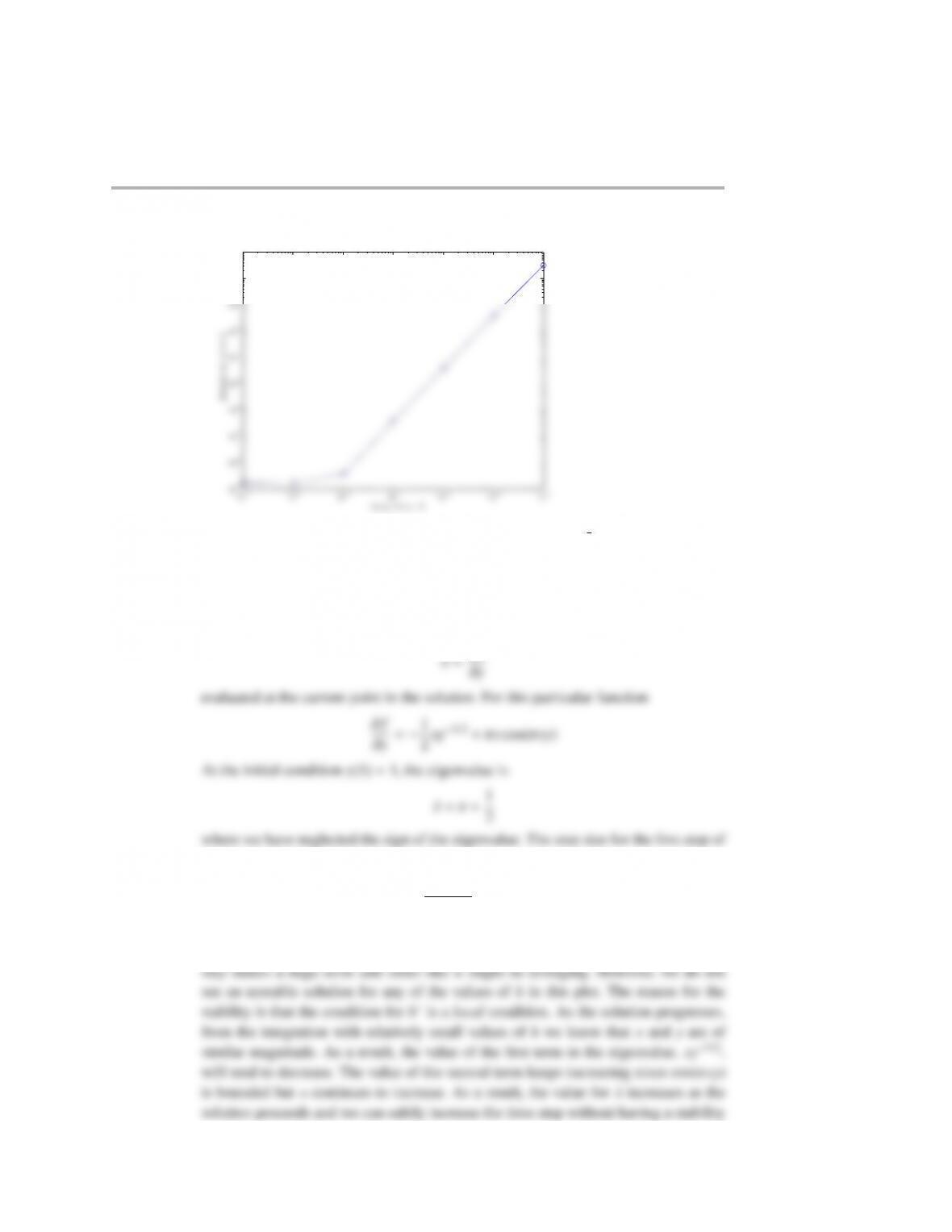
(4.35) The files for this problem are contained in the folder s12c8p2 matlab.
From the linear stability analysis, we know that the RK4 method requires a local
stability
hλ < 2.785
where the eigenvalue is approximated by
the integration then needs to be smaller than
h∗=2.785
π+1/2=0.7648
In the plot, the value for h∗is indeed stable for the first step and actually rather
accurate compared to the solution for h=0.01. When we exceed h∗, then the first
250 Initial value problems
problem. In this case, although there are stability issues at the start, the solution does
not blow up.
The Matlab script is:
1function s12c8p2
2close all
3clc
14
15 %make a figure for the plot
16 g = figure;
17 plot(x1,y1,‘-ob’,x2,y2,‘-og’,x3,y3,‘-or’)
18 axis([x0,xmax,y0,8])
0.1′,‘Location’,‘NorthWest’)
22 title(‘Solution for s12c8p2’,‘FontSize’,14)
23 saveas(g,‘s12c8p2 solution figure.eps’,‘psc2’)
24
25
36 y = rk4(x,y,h);
37 x = x+h;
38 %record the output for plotting
39 xplot(i+1) = x;
40 yplot(i+1) = y;