Unlock document.
This document is partially blurred.
Unlock all pages and 1 million more documents.
Get Access
Nonlinear equations 179
53 xlabel('$x$','FontSize',14)
54 ylabel('$y$','FontSize',14)
55 title('Solution to s13c6p3','FontSize',14)
56 saveas(g,'s13c6p123 solution figure3.eps')
67 J(1,2) = -y;
68 J(2,1) = P;
69 J(2,2) = -(1-y);
70 out = J;
The two output files are:
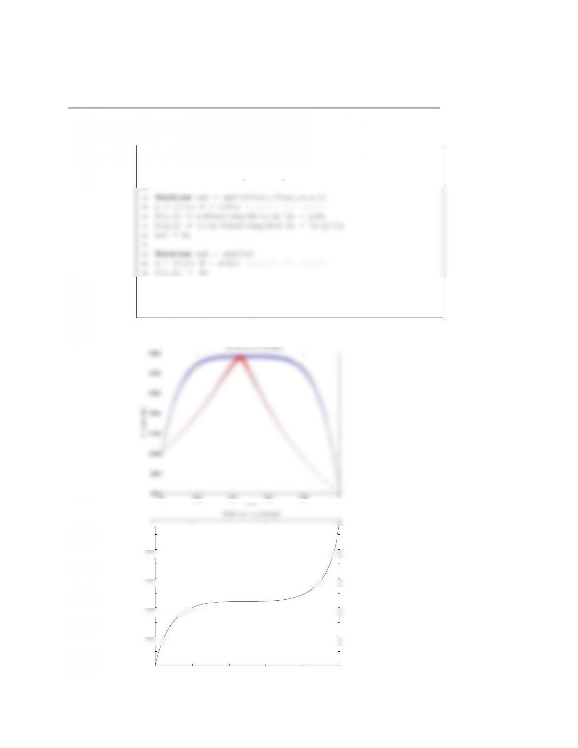
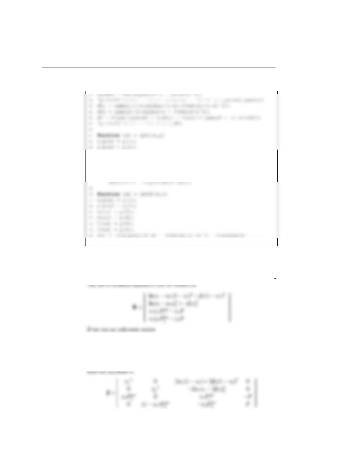
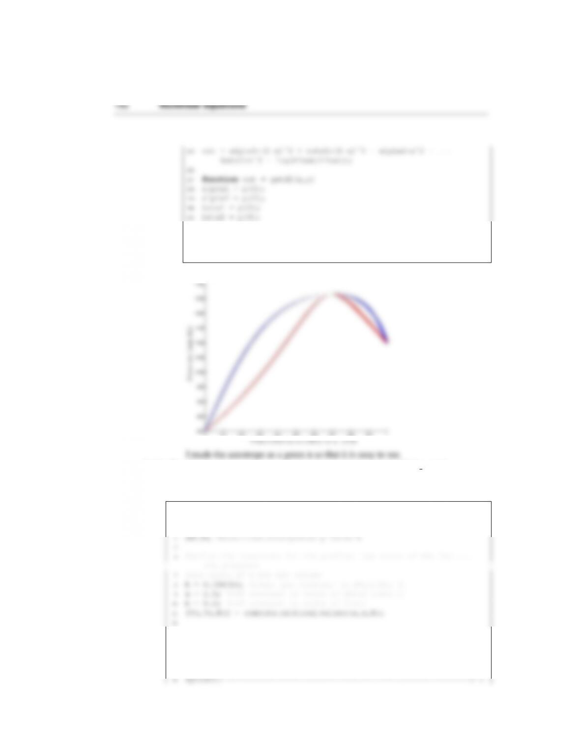
0 0.2 0.4 0.6 0.8 1
800
900
1000
1100
1200
1300
1400
1500
x, y
P(mm H g)
Solution t o s 13c 6p3
0 0.2 0.4 0.6 0.8 1
0
0.1
0.2
0.3
0.4
0.5
0.6
0.7
0.8
0.9
1
y
Solution to s13c 6p3
180 Nonlinear equations
Note on the thermodynamics problem. One nice thing about the one param-
eter model is that you can solve for the azeotrope without making a nonlinear
problem. The root of f(x1) is
2
problem 3.
1function out = s13c6p1 fast
2clc
3close all
4set(0,'defaulttextinterpreter','latex')
15 xlabel('$x {\mathrm{azeo}}$','FontSize',14)
16 ylabel('$P {\mathrm{azeo}}$','FontSize',14)
17 title('Solution to s13c6p1','FontSize',14)
18 saveas(h,'s13c6p1 fast plot.eps','psc2')
1function out = s13c6p3 fast
11 npts = 200;
12 x = linspace(0,1,npts); %values of x1
13 P = x.*exp(A*(1-x).ˆ2)*P1sat + (1-x).*exp(A*x.ˆ2)*P2sat;
14 y = x.*exp(A*(1-x).ˆ2)*P1sat./P;
15
26 ylabel('$y$','FontSize',14)
27 title('Solution to s13c6p3','FontSize',14)
28 saveas(g,'s13c6p3 fast plot2.eps','psc2')
Note that the solution here only works for the one-parameter model. While this
is the best way to solve the problem for a thermodynamics class, it gives you no
(3.31) (a) The files for this problem are contained in the folder solutions/s15c6p1 matlab.
At the azeotrope, x=y. If we divide the two equilibrium expressions we get
γ1
=Psat
2
1−β2x3
1−ln Psat
Psat
1
The derivative we need is
f′=−2α1(1 −x1)−3β1(1 −x1)2−2α2x1−3β2x2
8% beta1 = 0.1;
9% beta2 = 0.05;
10 % P1sat = 1100;
11 % P2sat = 800;
12
23 %put all the parameters into a vector for easy passing
24 p(1,1) = alpha1;
25 p(2,1) = alpha2;
26 p(3,1) = beta1;
27 p(4,1) = beta2;
38 f = getf(x,p);
39 k=k+1;
40 if k>20
41 fprintf('Did not converge.\n')
42 end
53 y=x*P1sat*gamma1/P;
54 fprintf('y = %8.6f\n',y)
55
56 %Check that this is the maximum pressure
Nonlinear equations 183
67 beta1 = p(3);
68 beta2 = p(4);
69 P1sat = p(5);
70 P2sat = p(6);
71 out = alpha1*(1-x)ˆ2 + beta1*(1-x)ˆ3 - alpha2*xˆ2 - ...
3*beta2*xˆ2;
The code is a bit more complicated than necessary, but I have set it up so that
it will be easier to use for later problems. The result is xazeo =0.744149 at
Pazeo =1138.5037 mm Hg.
(b) The files to solve this problem are contained in the folder solutions/s15c6p2 matlab.
x=
γ1
γ2
x1
y1
0 (1 −x1)Psat
2−γ2Psat
2P
The Matlab file to implement Newton-Raphson using the azeotrope as the initial
guess is:
184 Nonlinear equations
1function s15h6p2
2clc
13 P2sat = 800;
14 P = 1000; %junk value for now to put in place of pressure
15
16 %put all the parameters into a vector for easy passing
17 p(1,1) = alpha1;
24 %get the azeotope values from Problem #1
25 [x,P] = get azeotrope(p);
26 p(7,1) = P;
27
28 %set tolerance for Newton-Raphson
39
40 function [x,flag] = nonlinear newton raphson(x,tol,p)
41 % x = initial guess for x
42 % tol = criteria for convergence
43 % requires function R = getR(x)
54 J = getJ(x,p); %compute Jacobian
55 del = -J\R; %Newton Raphson
56 x = x + del; %update x
Nonlinear equations 185
57 k=k+1;%update counter
68 end
69
70
71 function out = getR(x,p)
72 %unpack the parameters for clarity
83 gamma2 = x(2);
84 x1 = x(3);
85 y1 = x(4);
86
87 %write equations
98 alpha1 = p(1);
99 alpha2 = p(2);
100 beta1 = p(3);
101 beta2 = p(4);
102 P1sat = p(5);
186 Nonlinear equations
113 J = zeros(4);
114 J(1,1) = 1/gamma1;
115 J(1,3) = 2*alpha1*(1-x1) + 3*beta1*(1-x1)ˆ2;
116 J(2,2) = 1/gamma2;
127 function [xvec,P] = get azeotrope(p)
128 %unpack parameters
129 alpha1 = p(1);
130 alpha2 = p(2);
131 beta1 = p(3);
142 x = x - f/df;
143 f = getf(x,p);
144 k=k+1;
145 if k>20
146 fprintf('Did not converge.\n')
157 %pack into Newton-Raphson vector
158 xvec(1,1) = gamma1;
159 xvec(2,1) = gamma2;
160 xvec(3,1) = x;
161 xvec(4,1) = x;
beta2*xˆ3 - log(P2sat/P1sat);
171
172 function out = getdf(x,p)
173 alpha1 = p(1);
174 alpha2 = p(2);
even if you gave a good guess, you will get a bad solution for δdue to a high
condition number, which means the new value of xmay not be better than the
previous guess. You can see how Newton-Raphson blows up when you set the
tolerance lower so that the while loop executes. There are tricks to handling
poorly conditioned matrices, but it seems unnecessary here since the residual is
2) or towards x1=1. Another option is to start from
cases very close to the pure species, where we know that the activity coefficients
are γ≈1 and the pressure is almost the saturation pressure. If you use this second
approach, you need to increase the pressure until you get near the azeotrope. I did
both approaches in this file to show you how it is done. In either case, be careful
10 alpha2 = A - 3*B;
11 beta1 = -4*B;
12 beta2 = 4*B;
188 Nonlinear equations
13 P1sat = 1100;
24 %get the azeotope values from Problem #1
25 [xazeo,Pazeo] = get azeotrope(p);
26 P = Pazeo;
27 p(7,1) = P;
28
38 x1 = xazeo-0.02;
39 y1 = xazeo-0.05;
40 gamma1 = exp(alpha1*(1-x1)ˆ2 + beta1*(1-x1)ˆ3);
41 gamma2 = exp(alpha2*x1ˆ2 + beta2*x1ˆ3);
42 x(1,1) = gamma1;
53 xleft(i) = x(3);
54 yleft(i) = x(4);
55 Pleft(i) = P;
56
57 fprintf('The solutions for P = %8.2f is\n',P)
Nonlinear equations 189
68 fprintf('***************************************\n')
69
70
71 %now start from almost pure species 2 and go up
82 npts = floor((Pazeo-Pmin)/dP);
83 xright = zeros(npts,1);
84 yright = zeros(npts,1);
85 Pright = zeros(npts,1);
86
97 fprintf('The solutions for P = %8.2f is\n',P)
98 fprintf(' gamma1 = %8.6f \n',x(1))
99 fprintf(' gamma2 = %8.6f \n',x(2))
100 fprintf(' x1 = %8.6f \n',x(3))
101 fprintf(' y1 = %8.6f \n',x(4))
111 ylabel('Pressure (mm Hg)','FontSize',14)
112 saveas(h,'s15h6p3 solution figure.eps','psc2')
113
114
115 function [x,flag] = nonlinear newton raphson(x,tol,p)
125 while norm(R) >tol
126 J = getJ(x,p); %compute Jacobian
127 del = -J\R; %Newton Raphson
128 x = x + del; %update x
129 k=k+1;%update counter
140 end
141
142 function out = getR(x,p)
143 %unpack the parameters for clarity
144 alpha1 = p(1);
155 x1 = x(3);
156 y1 = x(4);
157
158 %write equations
159 R = zeros(4,1);
170 alpha2 = p(2);
171 beta1 = p(3);
172 beta2 = p(4);
173 P1sat = p(5);
174 P2sat = p(6);
184 J = zeros(4);
185 J(1,1) = 1/gamma1;
186 J(1,3) = 2*alpha1*(1-x1) + 3*beta1*(1-x1)ˆ2;
187 J(2,2) = 1/gamma2;
188 J(2,3) = -2*alpha2*x1 - 3*beta2*x1ˆ2;
199 %unpack parameters
200 alpha1 = p(1);
201 alpha2 = p(2);
202 beta1 = p(3);
203 beta2 = p(4);
214 f = getf(x,p);
215 k=k+1;
216 if k>20
217 fprintf('Did not converge.\n')
218 end
229 alpha1 = p(1);
230 alpha2 = p(2);
231 beta1 = p(3);
232 beta2 = p(4);
233 P1sat = p(5);
242 P1sat = p(5);
243 P2sat = p(6);
244 out = -2*alpha1*(1-x) - 3*beta1*(1-x)ˆ2 - 2*alpha2*x - ...
3*beta2*xˆ2;
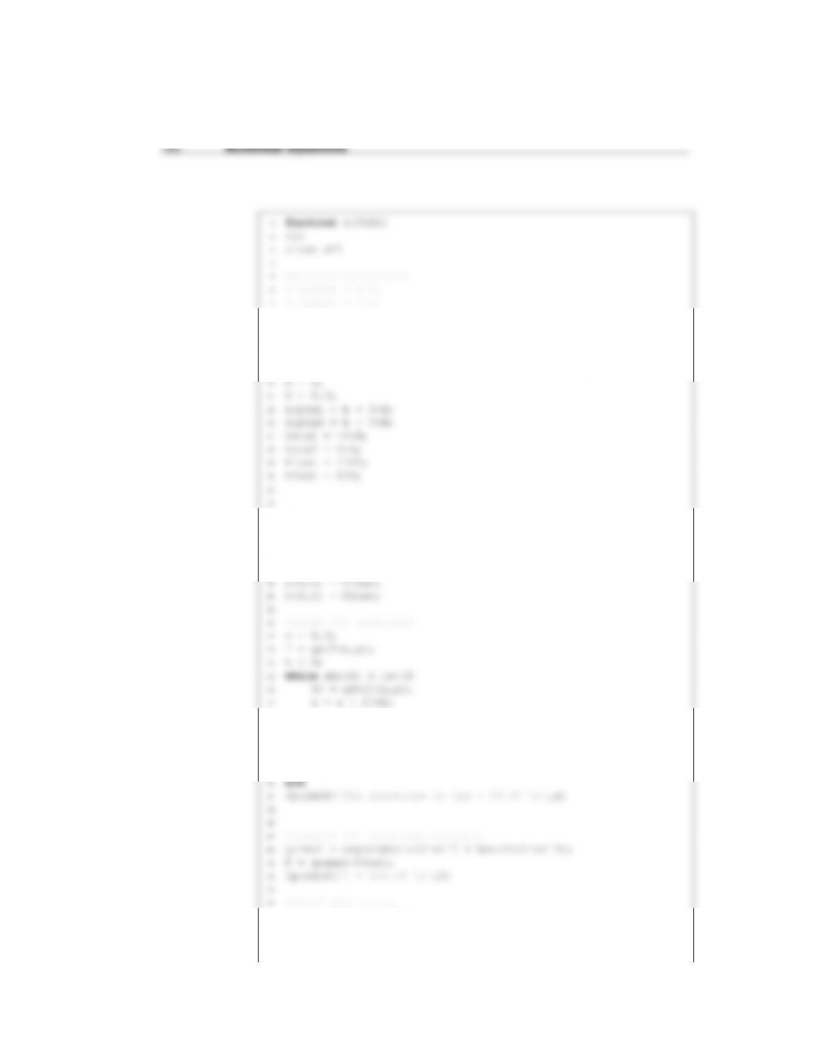
The output file is:
0 0.1 0.2 0.3 0.4 0.5 0.6 0.7 0.8 0.9 1
800
850
900
950
1000
1050
1100
1150
1200
1250
1300
C on c e nt rat i on x1( bl ue ) or y1( re d )
P r e ss ur e ( mm H g)
I made the azeotrope as a green xso that it is easy to see.
(3.32) The files for this problem are contained in the folder s12c5p12345 matlab.
The Matlab file that solves this entire problem is:
1function s12c5p12345
2clc
3close all
13
14 %%%%%%%%%%%%%%%%%%%%%%%%%%%%%%%%%%%%%%%%%%%%%%%%%%
15 %%% QUESTION #1
16 %%%%%%%%%%%%%%%%%%%%%%%%%%%%%%%%%%%%%%%%%%%%%%%%%%
17 fprintf('\n\n')
27 V guess = 0.5;
28 V = find V(P,V guess,T,a,b); %use Newton's method to find V
29 fprintf('V = %8.6f at P = %3.2f MPa and T = %6.2f K\n',V,P,T)
30
31
42 h = plot vdw(T,a,b,0.21,3,0,6);
43 saveas(h,'s12c5p12345 solution figure2a.eps','psc2')
44
45 %use a decent guess
46 V = 0.23;
57 fprintf('PROBLEM #3 \n')
58 fprintf('*****************************************************\n')
59
60 %use a bad guess
61 V = 0.6;
72 fprintf('\n\n')
73 fprintf('*****************************************************\n')
74 fprintf('PROBLEM #4 \n')

194 Nonlinear equations
75 fprintf('*****************************************************\n')
86 %compute the values of Vl, Vg and Psat at this T
87 [Vl,Vg,Psat] = equilibrium(P,T,Vl,Vg,a,b);
88 %plot the isotherm
89 h = plot isotherm(T,Vl,Vg,Psat,a,b);
90 saveas(h,'s12c5p12345 solution figure4b.eps','psc2')
101 %use the values from previous steps to make the phase envelope
102 fprintf('Generating phase envelope. Will output results at ...
each step.\n')
103 [g,h] = phase envelope(Pc,Vc,Tc,T,Psat,Vl,Vg,a,b);
104 saveas(h,'s12c5p12345 solution figure5a.eps','psc2')
114 Tc = (8*a)/(27*b*R);
115 Pc = (a/bˆ2)/27;
116
117 %display the results to the screen
118 fprintf('For a = %6.5f MPa Lˆ2/molˆ2 and b = %5.4f L/mol, \n',a,b)
Nonlinear equations 195
128 for i = 1:npts
129 P(i) = vdw(V(i),T,a,b);
130 end
131 h = figure;
the molar
142 %volume in L/mol and the temperature in K, a in in units of ...
MPa*Lˆ2/molˆ2
143 %and b in units of L/mol
144 R = 0.008314; %ideal gas constant in MPa*L/mol K
153 tol = 1e-8;
154 fVeval = fvdw(P,V,T,a,b); %value of function f(V)
155 k = 0; %counter
156 while abs(fVeval) >tol
157 V = V - fVeval/dfvdw(V,T,a,b);
167 out = V;
168
169 function [h,kcount,errcount] = find V plot(P,V,T,a,b)
170 %executes Newton's method to find a value of V in L/mol when ...
the vdw
the figure too.
176 Vinit = V;
177 tol = 1e-8;
178 fVeval = fvdw(P,V,T,a,b); %value of function f(V)
179 k = 0; %counter
190 fVeval = fvdw(P,V,T,a,b);
191 k = k+1;
192 kcount(k+1) = k;
193 Vcount(k+1) = V;
194 errcount(k+1) = abs(fVeval);
204 h=figure;
205 plot(kcount,Vcount,'-ob')
206 xlabel('Newton method iteration, $k$','FontSize',14)
207 ylabel('Value of molar volume, $\underline{V}ˆ{k}$...
(L/mol)','FontSize',14)
216 kscale(npts) = kcount(npts);
217 escale(npts) = errcount(npts);
218 for i = npts-1:-1:1
219 kscale(i) = kcount(i);
220 escale(i) = errcount(i+1)ˆ(1/2);
229 title(top,'FontSize',14)
230
231
232 function out = fvdw(P,V,T,a,b)
233 %computes the value of the vdw equation in the form f(V) = 0 ...
242 out = -R*T/(V-b)ˆ2+2*a/Vˆ3;
243
244 function out = plot Psat guess(P,T,a,b)
245 %make a plot of the initial guess. returns figure handle for ...
saving
256 axis([Vmin,Vmax,0,3])
257 xlabel('$\underline{V}$ (L/mol)','FontSize',14)
258 ylabel('$P$ (MPa)','FontSize',14)
259 top = strcat('Guess of Psat for $T = $',num2str(T),'K');
260 title(top,'FontSize',14)
270 Vg = find V(Psat,Vg,T,a,b);
271 fGeval = fGdep(Psat,Vl,Vg,T,a,b);
272
273 %start iterating
274 k = 1;
282 %update the volumes
283 Vl = find V(Psat,Vl,T,a,b);
284 Vg = find V(Psat,Vg,T,a,b);
285 %compute the new dG
286 fGeval = fGdep(Psat,Vl,Vg,T,a,b);
296
297 function out = fGdep(P,Vl,Vg,T,a,b)
298 %computes the difference in the departure Gibbs free energy ...
for the vdw
299 %equation with P in MPa, V in L/mol, T in K and returns dG in ...
309 out = (Vl-Vg);
310
311 function out = plot isotherm(T,Vl,Vg,Psat,a,b)
312 %create an isotherm below the critical point. returns handle ...
for plotting


