Unlock document.
This document is partially blurred.
Unlock all pages and 1 million more documents.
Get Access
Nonlinear equations 159
65 fprintf('Temperature difference at inlet is ...
\t%8.6f\n',T1-T1p)
66 fprintf('Temperature difference at outlet is ...
\t%8.6f\n\n',T2-T2p)
74 fprintf('*********************************************\n')
75 end
76
77
78 h = figure;
%6.4e\n',count,T2,abs(f))
91 while abs(f) >1e-6
%6.4e\n',count,T2,abs(f))
98 if count >100
99 fprintf('Did not converge! \n')
100 f = 0;
101 end
112 function out = getdf(T2,T1,T2p,p,a,b)
113 c = log((b + p*T2 - T2p)/(T2-T2p))*(p - 1);
160 Nonlinear equations
114 d = b-T2*(1-p);
115 e=p*(T2-T2p) - (b + p*T2 - T2p);
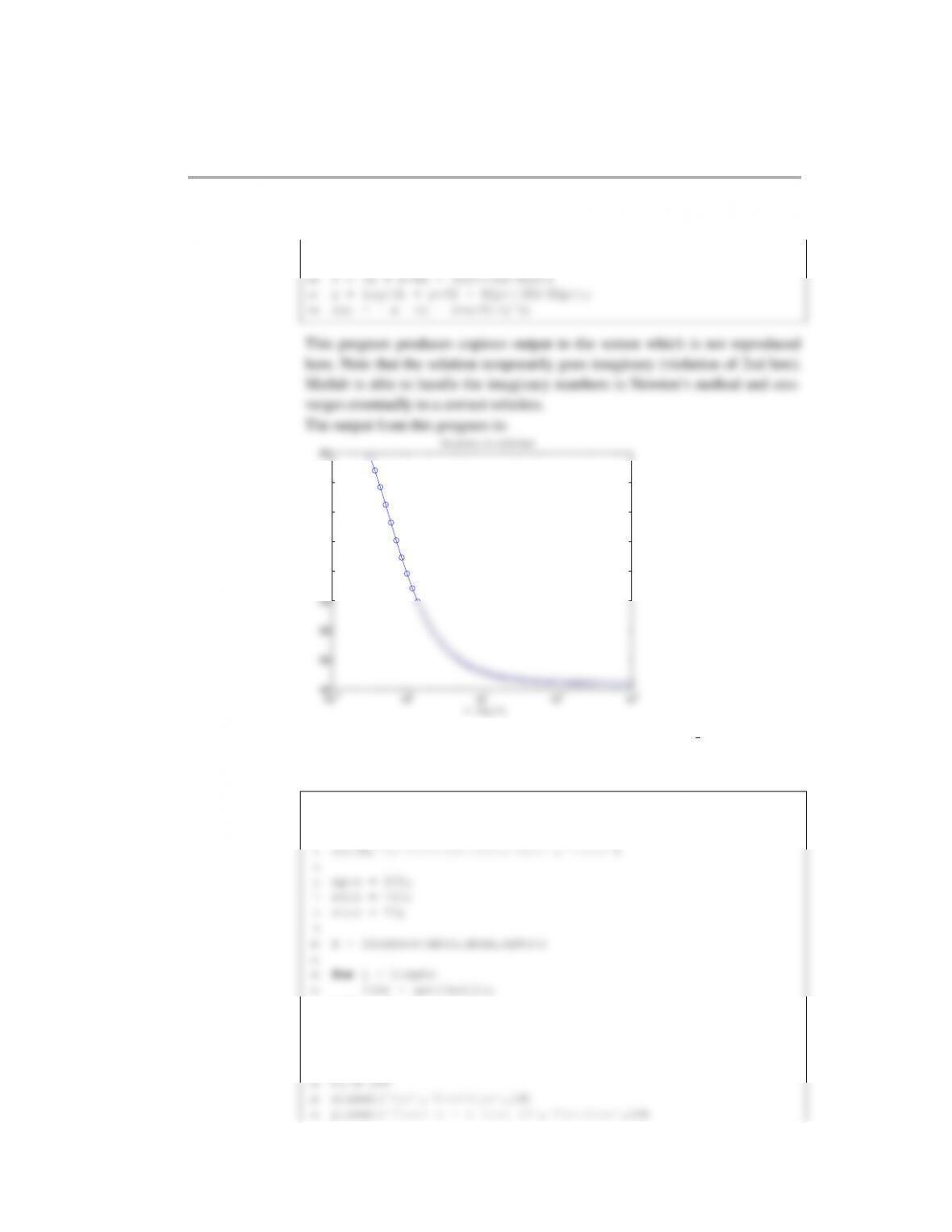
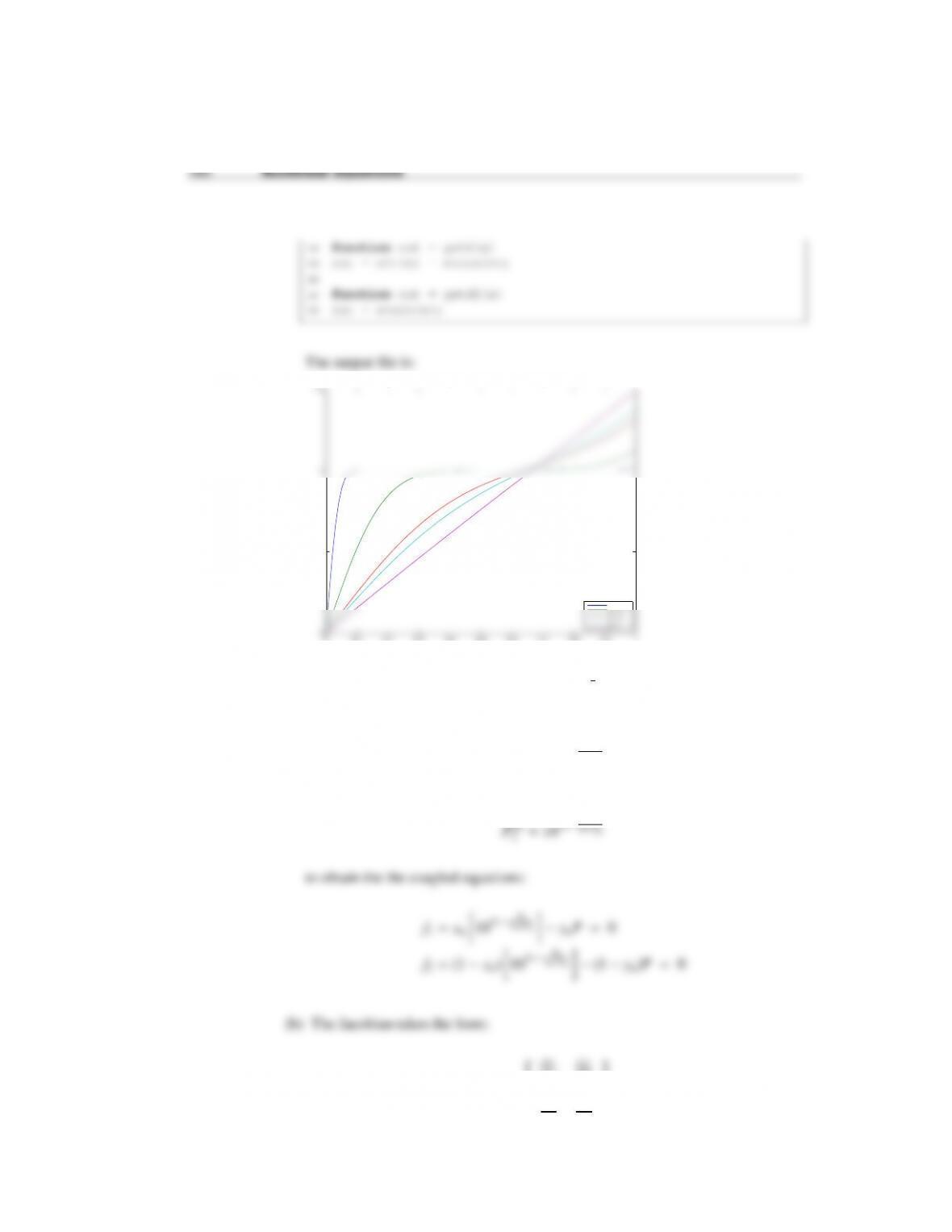
The output file is:
−10 −8 −6 −4 −2 0 2 4 6 8 10
−10
−8
−6
−4
−2
0
2
4
6
8
10
x
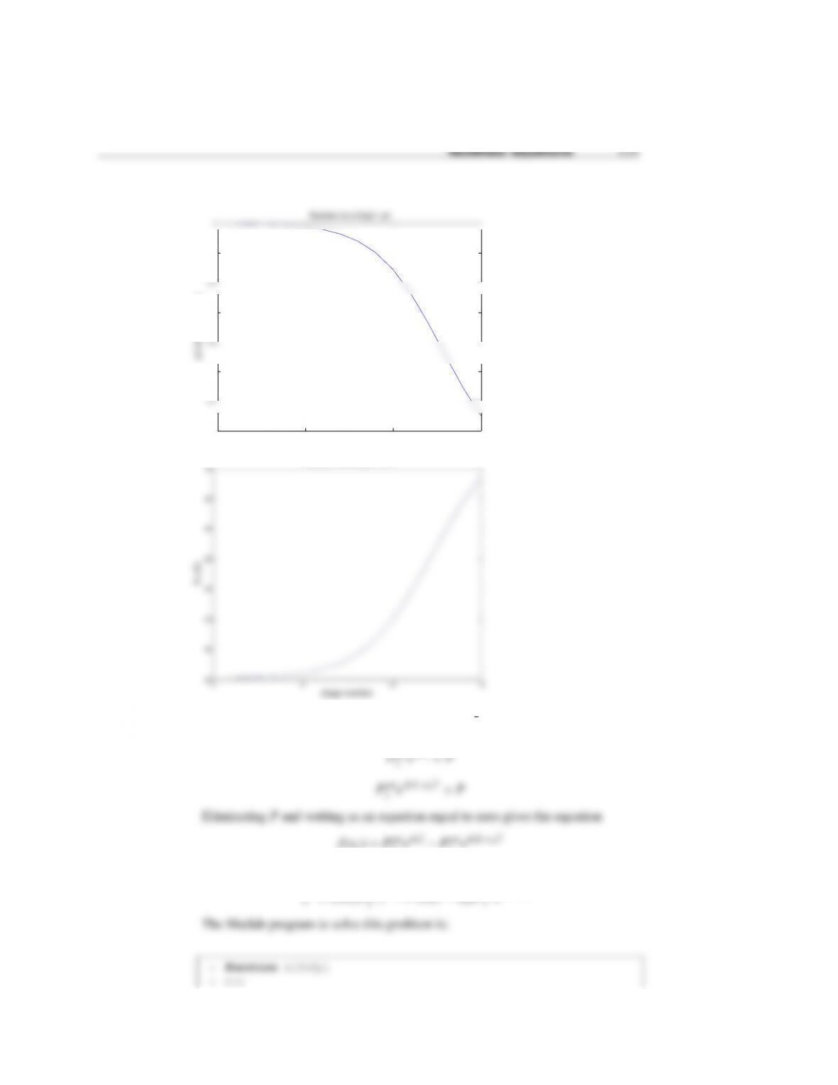
s i nx−xc osx
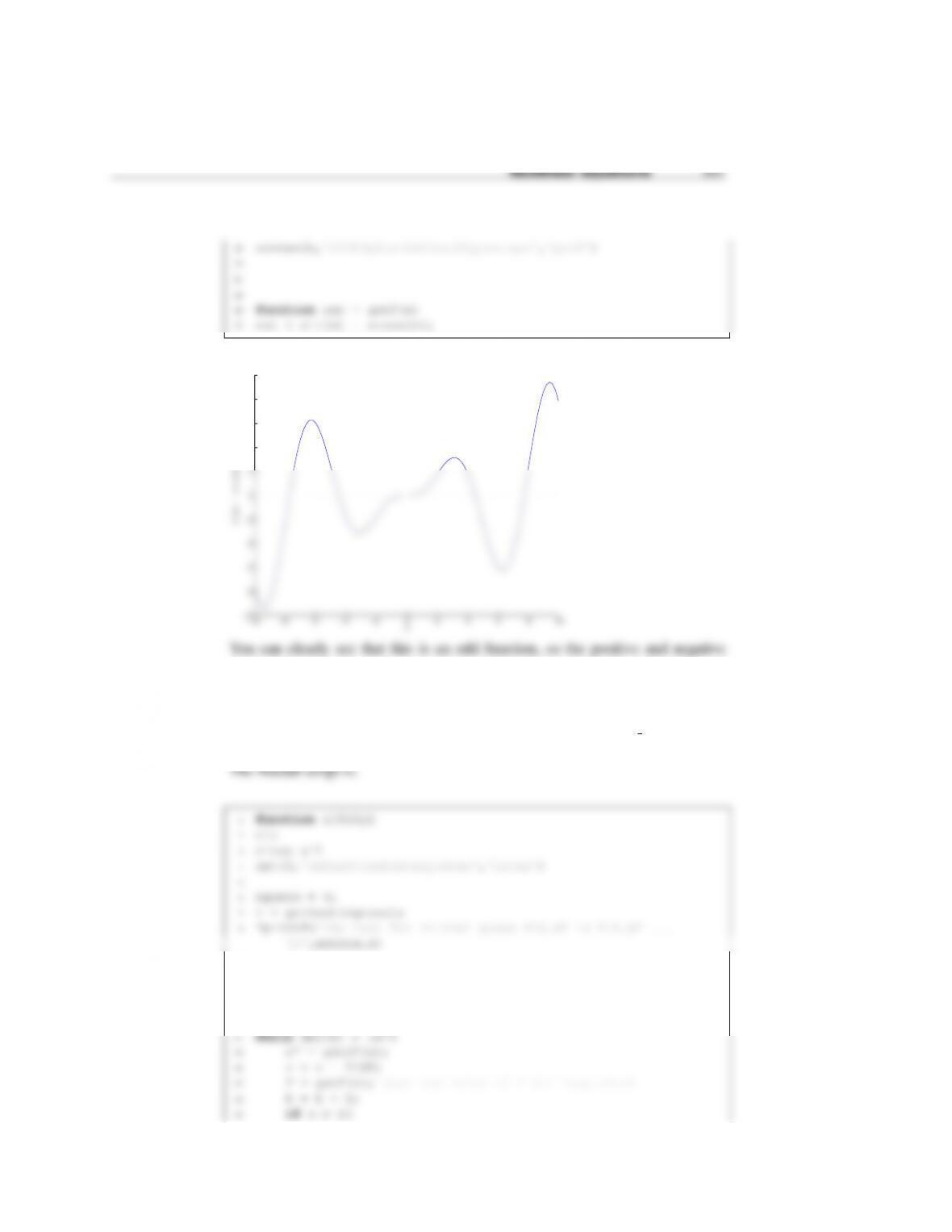
You can clearly see that this is an odd function, so the positive and negative
eigenvalues are of the same magnitude. I plotted the result with a dashed line at
x=0 to make it easier to see the roots. A reasonable guess for the first positive
eigenvalue is λ1=4.
(b) The files for this problem are contained in the folder s15c5p2 matlab. The
function is f(x)=sin x−xcos xand the derivative is f′(x)=xsin x.
9
10 function out = getRoot(x)
11 %use Newton's method with initial guess x
12 f = getf(x);
13 k = 0;
162 Nonlinear equations
25 out = x;
26
27 function out = getf(x)
28 out = sin(x) - x*cos(x);
29
30 function out = getdf(x)
31 out = x*sin(x);
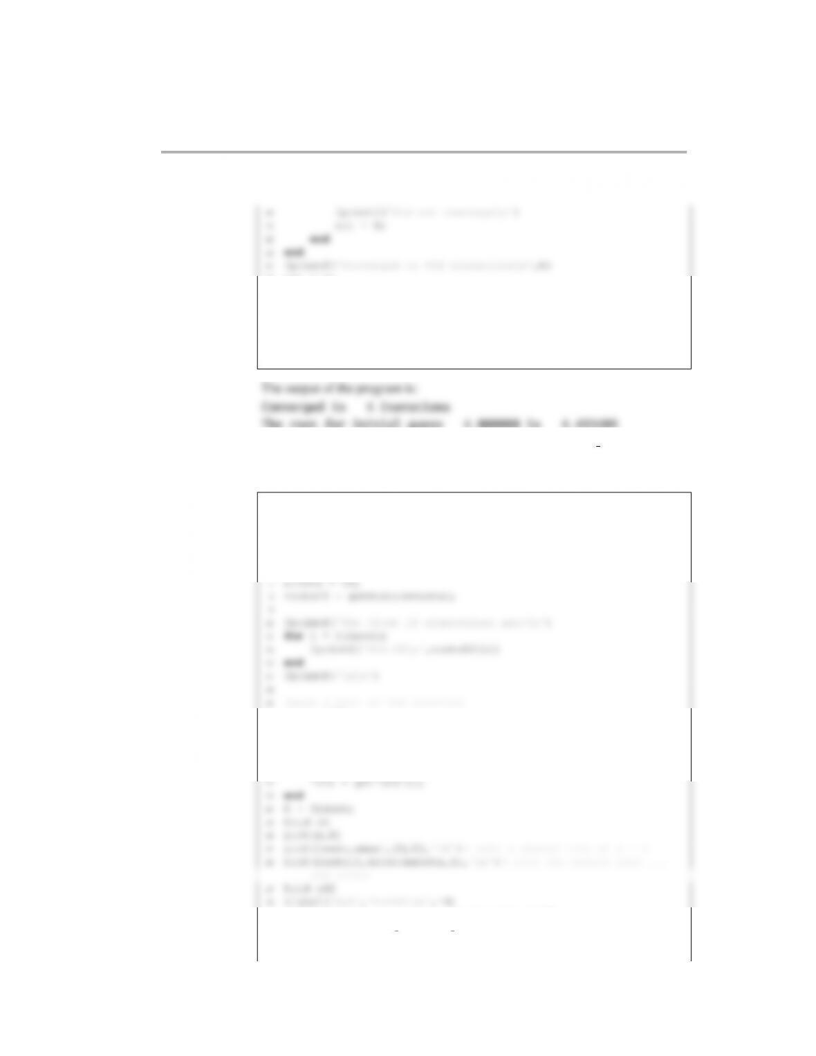
The root for initial guess 4.000000 is 4.493409
(c) The files for this problem are contained in the folder s15c5p3 matlab.
The Matlab script is:
1function s15h5p3
2clc
3close all
4set(0,'defaulttextinterpreter','latex')
5
6%get the first ten roots
17 npts = 101;
18 xmin = -0.1; % a bit before the trivial root
19 xmax = max(roots10) + 1; %slightly past the last root
20 x = linspace(xmin,xmax,npts);
21 for i = 1:npts
31 ylabel('$\sin x - x \cos x$','FontSize',14)
32 saveas(h,'s15h5p3 solution figure1.eps','psc2')
33
34 %get the first 150 roots
Nonlinear equations 163
45 xlabel('$n$','FontSize',14)
46 ylabel('$\lambda {n+1}-\lambda n$','FontSize',14)
47 saveas(h,'s15h5p3 solution figure2.eps','psc2')
48
49
60 fold = getf(xold);
61 nguesses = 0;
62 ngoal = nroots-1; %find 9 more good guesses
63 xguess = zeros(ngoal,1);
64 while nguesses <ngoal
75 fold = fnew; %store for next step
76 if xnew >500
77 nguesses = 100;
78 end
79 end
89
164 Nonlinear equations
90
91 function out = getRoot(x)
92 %use Newton's method with initial guess x
103 end
104 end
105 out = x;
The first ten eigenvalues are
4.493409
10.904122
17.220755
23.519452
29.811599
32.956389
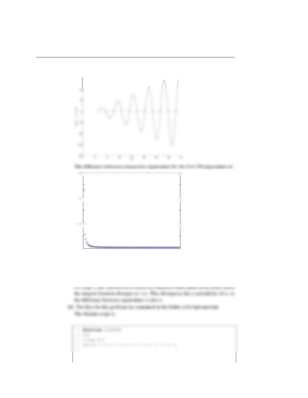
To see that these are indeed the right results, I also made a plot:
Nonlinear equations 165
−5 0 5 10 15 20 25 30 35
−40
−30
−20
−10
0
10
20
30
x
s i nx−xc osx
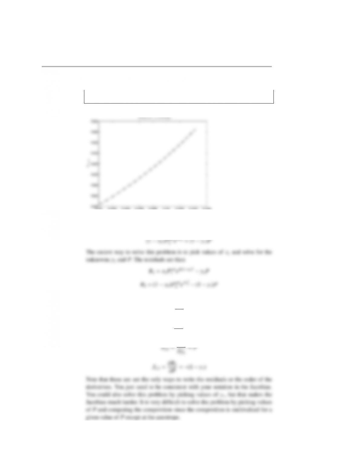
The difference between consecutive eigenvalues for the first 150 eigenvalues is:
0 50 100 150
3.14
3.16
3.18
3.2
3.22
3.24
3.26
n
λn+ 1−λn
For large x, the eigenvalues are spaced by a distance of π. The reason is easiest
to see if you think about the eigenvalue equation as
x=tan x
6%call the results of problem 3 to get the first n roots
7nroots = 150;
166 Nonlinear equations
8dx = 0.01;
9xguess = 4;
20 for j = 1:npts
21 xpt = x(j);
22 output(i,j) = getc(xpt,tpt,lambda);
23 end
24 end
35 s = 0;
36 for i = 1:length(lambda)
37 L = lambda(i);
38 cn = 4*(1-cos(L))/(2*L-sin(2*L));
39 s=s+cn*sin(L*x)*exp(-Lˆ2*t);
50 %scan through the function by bracketing for good guesses
51 dx = 0.1;
52 xold = r;
53 fold = getf(xold);
54 nguesses = 0;
64 nguesses = nguesses + 1;
65 xguess(nguesses) = xnew;
66 end
67 xold = xnew; %store for next step
68 fold = fnew; %store for next step
78
79 roots
80
81
82 %make a plot of the function
93 plot([xmin,xmax],[0,0],':k')% make a dashed line at x = 0
94 plot(roots,zeros(nroots,1),'or')% plot the points that are ...
roots
95 hold off
96 xlabel('$x$','FontSize',14)
107 df = getdf(x);
108 x = x - f/df;
109 f = getf(x); %get new value of f for loop check
110 k=k+1;
111 if k>20
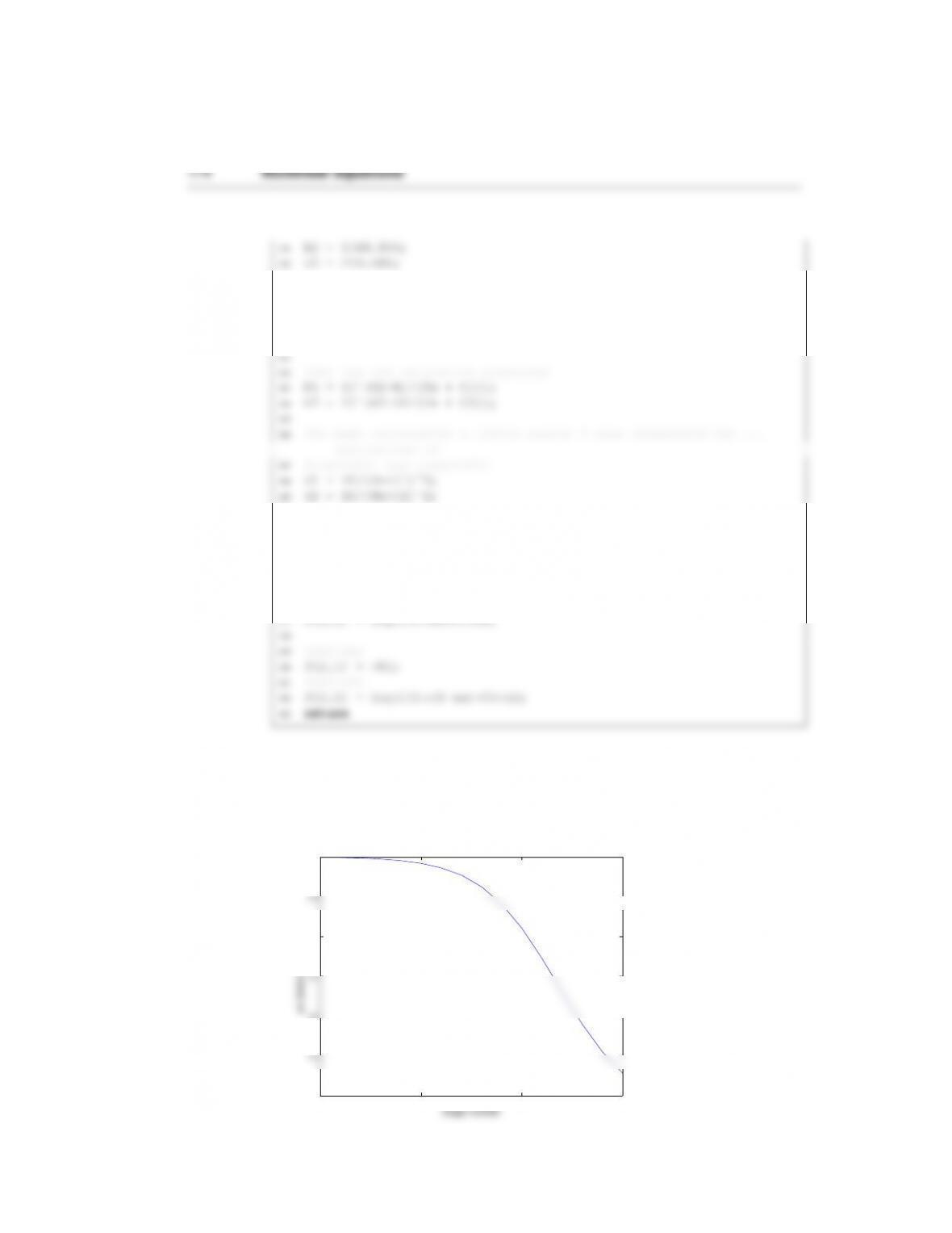
0 0.1 0.2 0.3 0.4 0.5 0.6 0.7 0.8 0.9 1
0
0.5
1
1.5
x
c
0 . 0 0 0 5
0 . 0 1
0 . 0 5
0 . 0 7
0 . 2
(3.29) The files for this problem are in the folder s10cp1 matlab.
(a) Rearrange:
Psat
1=10A1−B1
Tn+C1
Tn+C2
J=
∂xn
∂Tn
∂f2
∂xn
∂f2
∂Tn
Nonlinear equations 169
∂xn
=−10A2−B2
Tn+C2
∂f2
=(1 −xn)10A2−B2
Tn+C2ln 10 "B2
∂f2
∂xn
∂f2
∂Tn
−406.7 3.945 #
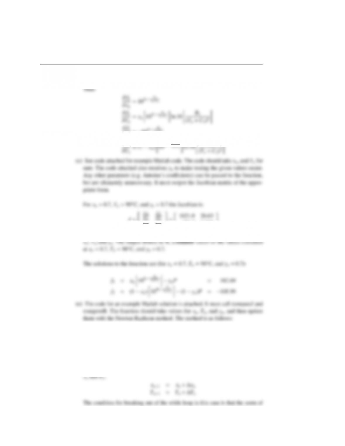
(d) The code for an example Matlab function is attached. Again, it should be given
Jn(xn+1−xn)=−Rn
This can then be simplified to:
δ="∆xn
∆Tn#=−J\R
The backslash is the Matlab command. The values in δcan be used to update for
xn
yn
Tn
=
0.4839
0.7
92.5815
To hand-check:
Tn+C1−ynP=−0.0419
Tn+C2−(1 −yn)P=0.0168
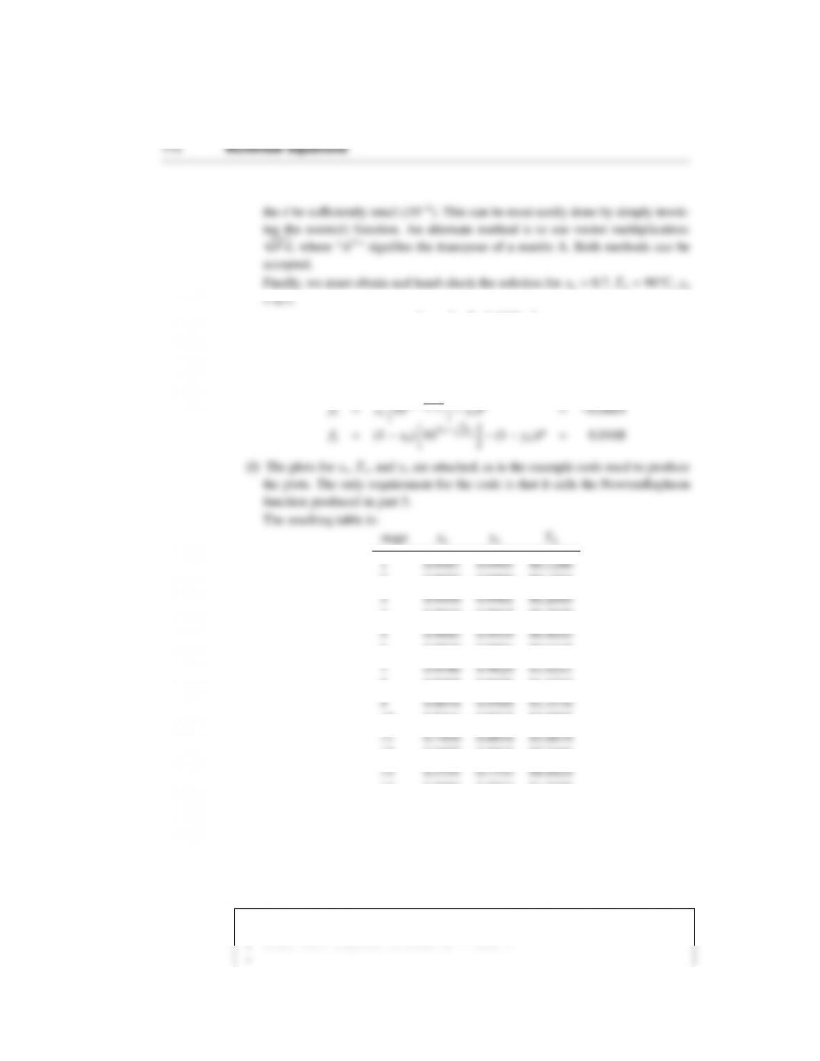
2 0.9973 0.9990 80.1534
4 0.9910 0.9965 80.2805
6 0.9730 0.9894 80.6445
8 0.9255 0.9698 81.6262
10 0.8211 0.9217 83.8992
12 0.6607 0.8313 87.7466
14 0.5096 0.7216 91.8358
15 0.4564 0.6756 93.4018
Note that the ynis not updated using NewtonRaphson.
The Matlab script for this problem is:
1%rectification
2%Patrick Smadbeck
9%The result is then outputed and also plotted against the ...
stage number
10
11 %Inputs: none
12
determine the
20 %rectification line
21 N = 15;
22 Rd = 1.95;
23 xD = 0.9995;
32
33 %Here are the initial guesses. I give both mole fractions as ...
xD, and then
34 %Tn as the boiling point of Benzene
35 xn = xD;
45 for k = 1:N
46 %Get the result for stage k
47 x = NewtonRaph(x);
48 %Add it to the matrix
172 Nonlinear equations
58 %It is also platted for each
59 n = 1:N;
60
61 h=figure;
62 plot(n,xM(:,1));
73 saveas(h,'s10cp1 solution figure2.eps','psc2')
74
75
76 h=figure;
77 plot(n,xM(:,3));
88 %These are guesses. It is based on zeroth order continuation, ...
which simply
89 %means the solution to the previous stage is the guess for the ...
next
90
Nonlinear equations 173
101 %Update xn and Tn (yn will remain the same since it is not ...
specified in
102 %the Jacobian file).
103 x(1) = x(1) + dx(1);
114 A1 = 6.90565;
115 B1 = 1211.033;
116 C1 = 220.790;
117
118 %TOLUENE
128 yn = x(2);
129 Tn = x(3);
130
131 %Here the saturated pressures are calculated to make the ...
calculation nicer
142
143 function J = computeJ(x)
144 %x = [xn,yn,Tn];
145
146 %Antoine coefficients, given in the problem statement
156
157 %need xn, yn, and Tn
158 xn = x(1);
159 yn = x(2);
160 Tn = x(3);
170
171 %The Jacobian will be 2X2
172 J = zeros(2);
173
174 %Here is df1/dxn
175 J(1,1) = P1;
176 %Here is df1/dTn
177 J(1,2) = log(10)*xn*P1*d1;
The output files are
0 5 10 15
0.4
0.5
0.6
0.7
0.8
0.9
1
Solution to s10cp1: xn
stage number
0 5 10 15
0.65
0.7
0.75
0.8
0.85
0.9
0.95
1
Solution to s10cp1: yn
stage number
yn (mole fraction)
0 5 10 15
80
82
84
86
88
90
92
94
Solution to s10cp1: Tn
stage number
Tn (C)
(3.30) The files for this problem are in the folder s13c6p123 matlab.
(a) The azeotrope corresponds to the condition
2eAx2
1eA(1−x1)2
The derivative for Newton’s method is
f′=2Ax1Psat
1+2A(1 −x1)Psat
176 Nonlinear equations
11 Pazeo = zeros(npts,1); %memory for azeotrope pressures
12 xazeo = zeros(npts,1); %memory for azeotrope composition
22 end
23
24 h = figure;
25 plot(xazeo,Pazeo,'-ok','MarkerSize',8)
26 xlabel('$x {\mathrm{azeo}}$','FontSize',14)
%6.4e\n',k,x,err);
42 if k>10
43 fprintf('\t Did not converge!')
44 end
45 end
56 function out = getP(P2sat,A,x)
Nonlinear equations 177
57 %x = x1
58 out = P2sat*exp(A*xˆ2);
The output figure is:
0.43 0.432 0.434 0.436 0.438 0.44 0.442 0.444 0.446
1340
1360
1380
1400
1420
1440
1460
1480
1500
xa z e o
Pa z e o
Solution t o s 13c6p1
(b) The equilibrium conditions are
x1Psat
1eA(1−x1)2=y1P
2eAx2
With this form of the residuals and order of the unknowns, the Jacobian is
J1,1=∂R1
∂y1
=−P
J1,2=∂R1
∂P
=−y1
178 Nonlinear equations
(c) The Matlab script to solve this problem is:
1function s13c6p3
2clc
3close all
14
15 %input the endpoints
16 yplot(1) = 0; Pplot(1) = P2sat; %values when x1 = 0
17 yplot(npts) = 1; Pplot(npts) = P1sat; %values when x1 = 1
18
28 J = getJ(z);
29 delta = -J\R;
30 z = z + delta;
31 R = getR(P1sat,P2sat,A,x,z);
32 err = norm(R);
43
44 h = figure;
45 plot(xplot,Pplot,'ob',yplot,Pplot,'or')
46 xlabel('$x,y$','FontSize',14)
47 ylabel('$P$ (mm Hg)','FontSize',14)


