Introduction 25
15 for l = 1:n
16 A(k,l) = (k+l)/(k*l);
17 end
18 end
29 output
30
31 function out = transp(A,m,n)
32 %A = original matrix with m rows and n columns. create transpose
33 Atrans = zeros(n,m); %initialize as n x m matrix
44 %A = left matrix with m x n
45 %B = right matrix with n x m
46 C = zeros(m,m); %initialize output matrix
47 for i = 1:m
48 for j = 1:m
59 %compute the trace of an mxm matrix
60 tr = 0; %initialize as zero
61 for i = 1:m
62 tr = tr + C(i,i);
63 end
64 out = tr;
The output is:
(1.38) The files for this problem are contained in the folder s11c2p1 matlab.
The Matlab script is:
1function s11c2p1
2close all
3clc
14 result = big number;
15 for i = 1:10ˆj
16 result = result + small number;
17 end
18 result = result-big number;
Introduction 27
10−10 10−9 10−8 10−7 10−6 10−5 10−4 10−3 10−2 10−1
0
0.2
0.4
0.6
0.8
1
1.2
1.4
1.6
1.8
2
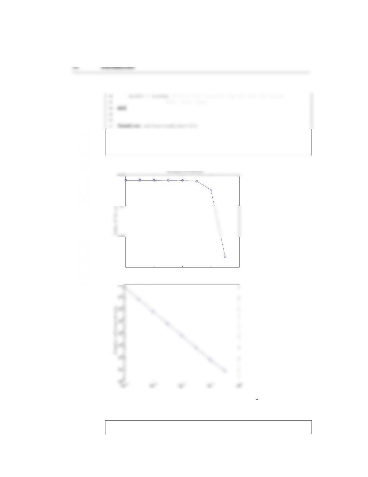
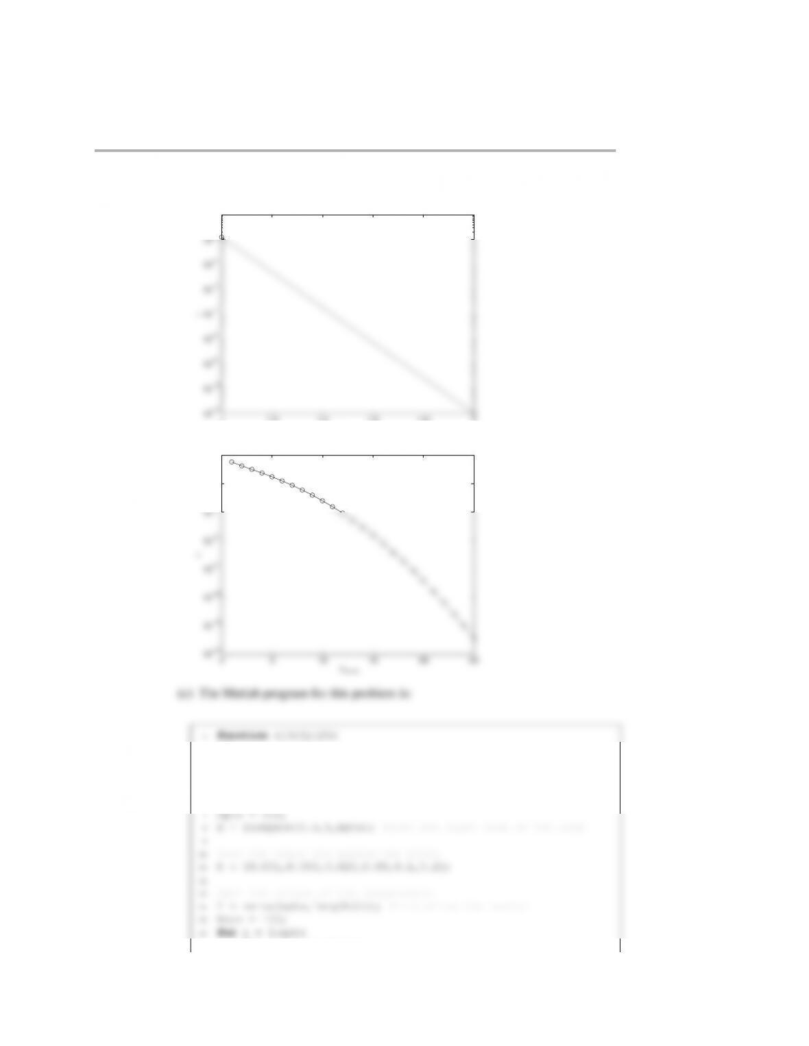
Solution t o s11c2p1
²
Result
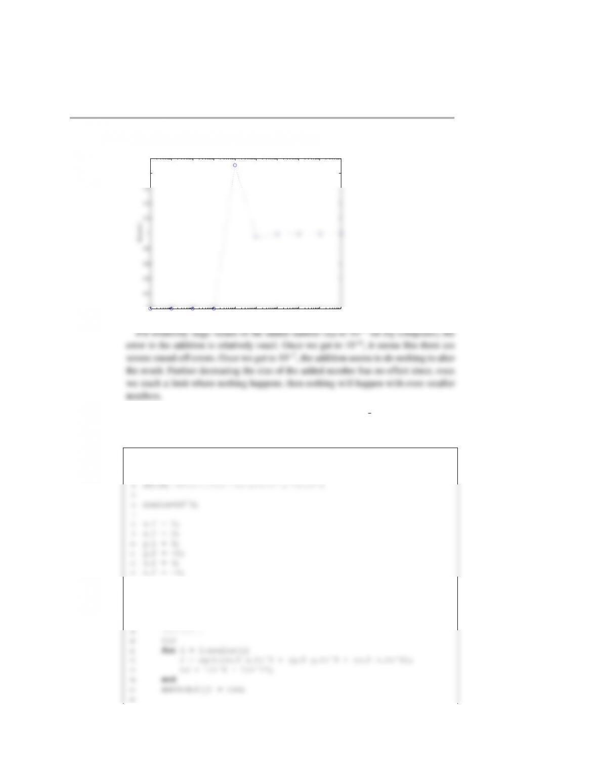
For relatively large values of the added number (up to 10−5on my computer), the
error in the addition is relatively small. Once we get to 10−6, it seems like there are
severe round-offerrors. Once we get to 10−7, the addition seems to do nothing to alter
the result. Further decreasing the size of the added number has no effect since, once
we reach a limit where nothing happens, then nothing will happen with even smaller
numbers.
(1.39) The files for this problem are contained in the folder s12c3p2 matlab.
The Matlab script is:
1function s12c3p2
2clc
3close all
14
15
16 for j = 1:8
17 ncalcs(j) = 10ˆj;
18
28 for i = 1:ncalcs(j)
29 r2 = (x 2 –x 1)ˆ2 + (y 2–y 1)ˆ2 + (z 2 –z 1)ˆ2;
30 r2inv = 1/r2;
31 r6inv = r2inv*r2inv*r2inv;
32 r12inv = r6inv*r6inv;
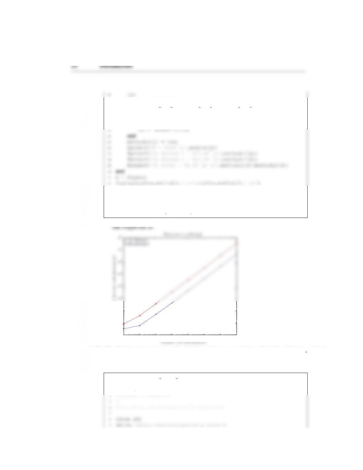
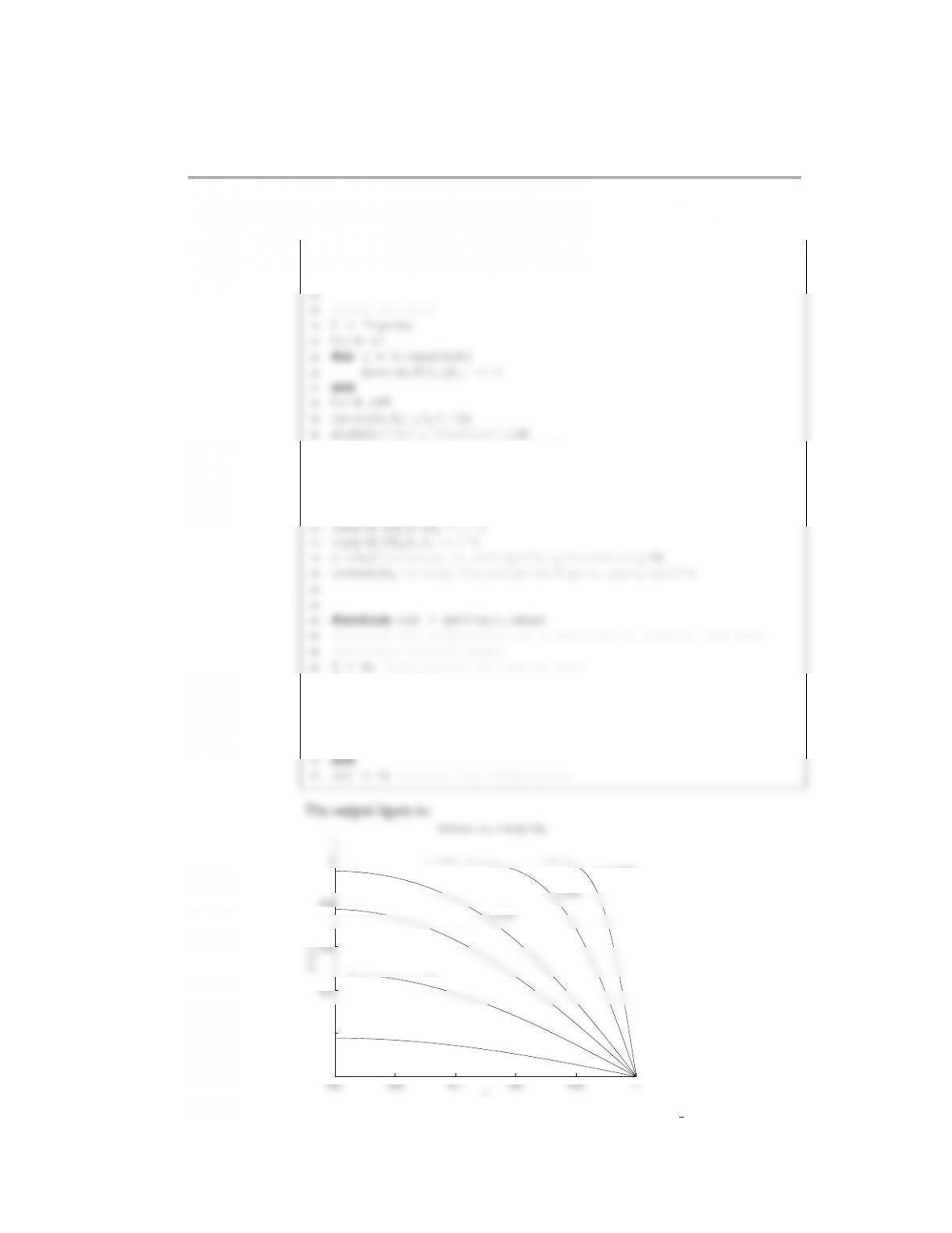
43 legend(‘Method 1’,‘Method 2’,‘Location’,‘NorthWest’)
44 xlabel(‘Number of calculations’,‘FontSize’,14)
45 ylabel(‘Time for the calculation (s)’,‘FontSize’,14)
46 title(‘Solution to s12c3p2’,‘FontSize’,14)
47 saveas(h,‘s12c3p2 solution figure.eps’,‘psc2’)
101102103104105106107108
10−6
10−5
10−4
10−3
10−2
10−1
100
101
102
Numb e r of calc ulations
T im e f or t he c alc ula tio n ( s)
Solution t o s12c 3p2
M e t h o d 1
M e t h o d 2
(1.40) The Matlab script and output files for this problem are available in the folder s10c1p1 matlab.
1function [value sum,n terms]= s10c1p1
2%the output for this value is
3%value sum = 3.141592637882101
13 %the value of N is the max on a log scale
14 N = 8;
15
16 %initialize the variables
17 k = 0;
28 %continuing from the last iteration
29 [x old,k] = compute sum(epsilon(i),x old,k);
30
31 %store the output values from the iteration
32 output(i) = x old;
43
44 h=figure;
45 loglog(epsilon,terms,‘-o’,‘MarkerSize’,8)
46 xlabel(‘$\epsilon$’,‘FontSize’,14)
47 ylabel(‘Number of terms in sum’,‘FontSize’,14)
58 %It takes the value of the sum (x old) and the last term (k)
59 %from the previous value of epsilon to increase the speed
60 %of the program.
61 error = 1000;
62 while error >epsilon
72 %this subfunction computes the current term in the summation
73 numerator = 2*mod(i,2)-1; %this is faster than -1ˆ(k+1)
74 denominator = 0.5*i-0.25;
75 out = numerator/denominator;
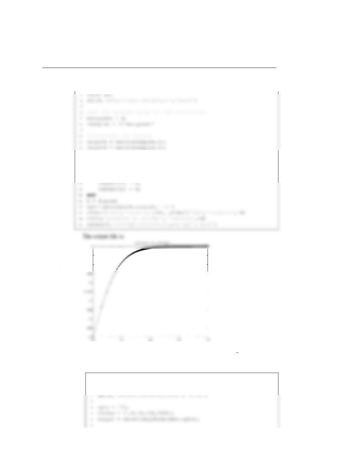
The output files are:
10−8 10−6 10−4 10−2 100
3
3.05
3.1
3.15
²
Value of the sum
Solution to s10c1p1
10−8 10−6 10−4 10−2 100
100
101
102
103
104
105
106
107
108
²
Numbe r of te rms in sum
Solution to s10c 1p1
(1.41) The files for this problem are contained in the folder s12c3p1 matlab.
1function s12c3p1
2clc
Introduction 31
13
14 S = 0; %initialize the sum
15
16 for n = 1:nsamples
17 S = S + 1/(n+1)/n;
32 Introduction
10 x = linspace(0,1,npts);
11 t =0;
12
13 for i = 1:length(nmodes)
14 ncurrent = nmodes(i);
15 for j = 1:npts
16 xpt = x(j);
17 output(i,j) = getc(xpt,t,ncurrent);
28 c = 0;
29 for k = 0:n
30 L = (2*k+1)*pi/2;
31 c=c+2*(-1)ˆk/L *cos(L*x) *exp(-Lˆ2*t);
32 end
0 0.1 0.2 0.3 0.4 0.5 0.6 0.7 0.8 0.9 1
0
0.2
0.4
0.6
0.8
1
1.2
1.4
x
c
1
5
1 0
1 0 0
1 0 0 0
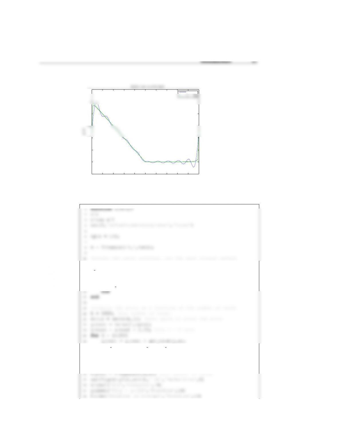
The accuracy improves as we increase the number of modes k. We always have
great accuracy at x=0 because the cosine function is unity there. The problem
is at x=1 because we are trying to add a bunch of functions with zero value
5
6npts = 101;
7nmodes = 20;
8
9x = linspace(0,1,npts);
20 end
21 plot(x,c,‘-k’)
22 end
23 hold off
24 axis([0,1,0,1.05])
35 L = (2*k+1)*pi/2;
36 c=c+2*(-1)ˆk/L *cos(L*x) *exp(-Lˆ2*t);
37 end
38 out = c;
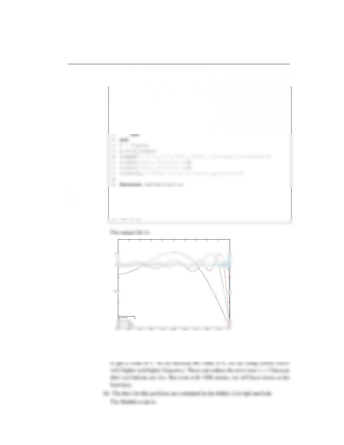
The output file is:
0 0.1 0.2 0.3 0.4 0.5 0.6 0.7 0.8 0.9 1
0
0.1
0.2
0.3
0.4
0.5
0.6
0.7
0.8
0.9
1
x
c
0 . 0 0 1
0 . 0 1
0 . 0 5
0 . 2 5
0 . 5
1
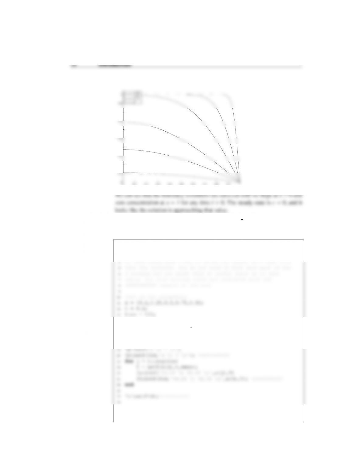
We can see that the boundary conditions are satisfied with no slope at x=0 and
zero concentration at x=1 for any time t>0. The steady-state is c=0, and it
looks like the solution is approaching that value.
(1.43) The solutions to this problem are in the folder s13c3p123 matlab.
(a) The Matlab file for this problem is
1function s13c3p123a
2clc
3
14
15 fid = fopen(‘s13c3p123a data.txt’,‘w+’); %XXXXXXXXXX
16
17 %compute the temperature
18 fprintf(‘Compute the temperatures at t = %3.2f\n’,t)
29
31 %returns the temperature at a position x, time t, and kmax
Introduction 35
32 %non-zero Fourier modes
33 T = 0; %initialize the sum at zero
34 for k = 1:kmax
The output of the file is
1x T
20.10 0.146691
40.50 0.474487
60.90 0.146691
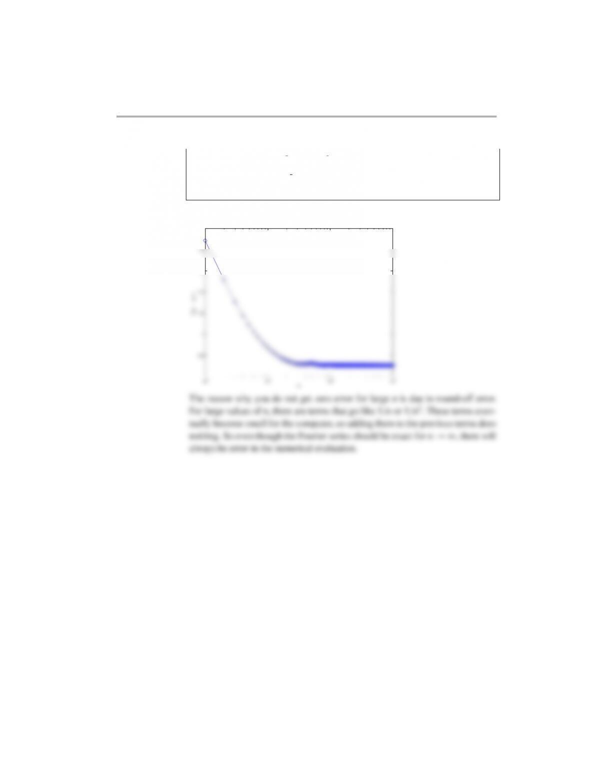
(b) The Fourier series converges very quickly, especially at long times (because
there is an exponential with n2. For t=0.1, you are already within machine
precision at the third Fourier mode. For shorter times, where the solution is more
flat, you need many Fourier modes to get convergence. For example, I made a
6
7
8%set the time
9t = 0.1;
10 [kplot,err] = get answer(t);
21 t = 0.001;
22 [kplot,err] = get answer(t);
23 %make a plot of the error versus Fourier modes
36 Introduction
24 h = figure;
35
36 %get the “exact value”
37 kexact = 100;
38 for j = 1:npts
39 Texact(j) = getT(x(j),t,kexact);
50 end
51 err(k) = norm(T-Texact)/norm(Texact);
52 end
53 kplot = linspace(1,kcount,kcount); %for plotting
54
65 out = T; %return the temperature
The output figures from the program are
Introduction 37
1 1.2 1.4 1.6 1.8 2
10−11
10−10
10−9
10−8
10−7
10−6
10−5
10−4
10−3
km a x
²
Solution to s13c 3p123b, t = 0.1
0 5 10 15 20 25
10−14
10−12
10−10
10−8
10−6
10−4
10−2
100
km a x
²
Solution to s13c 3p123b, t = 0.001
2clc
3close all
4set(0,‘defaulttextinterpreter’,‘latex’)
5
6%set up the vector for x
17 for j = 1:length(t)
38 Introduction
18 T(i,j) = getT(x(i),t(j),kmax);
19 end
20 end
31 ylabel(‘$T(x,t)$’,‘FontSize’,14)
32 text(0.93,0.95,‘$t$ = 0.001’)
33 text(0.87,0.85,‘0.005’)
34 text(0.76,0.75,‘0.025’)
35 text(0.7,0.65,‘0.05’)
46 for k = 1:kmax
47 n=2*k-1; %convert back to n notation so that
48 %this counts the odd terms
49 T = T + 4/(n*pi)*sin(n*pi*x)*exp(-nˆ2*piˆ2*t);
50 %term in series
Introduction 39
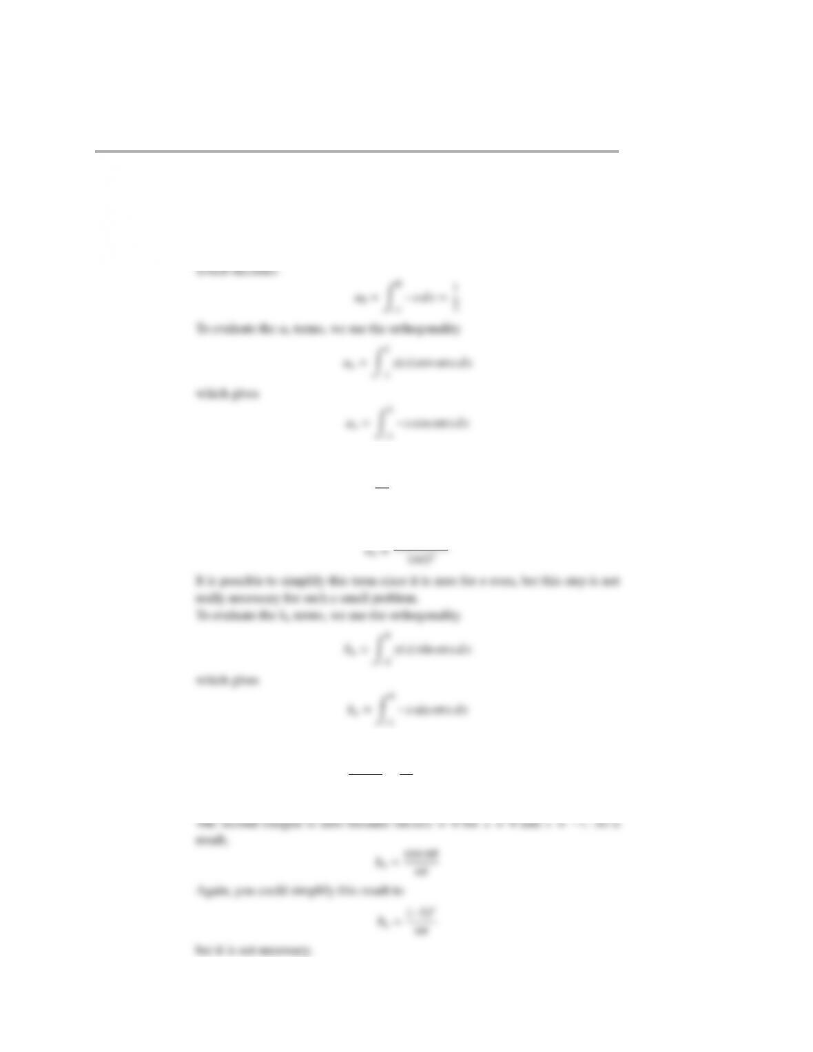
(a) The a0term is
a0=Z1
−1
y(x)dx
−1
Integrating once by parts gives
an=1
nπZ0
−1
sin nπx dx
because sin nπx=0 for x=0 and x=−1. The second integration gives
−1
Integrating once by parts gives
bn=cos nπ
nπ
−1
nπZ0
−1
cos nπx dx
where I have used the even property of the cos function, cos(−nπ)=cos(nπ).
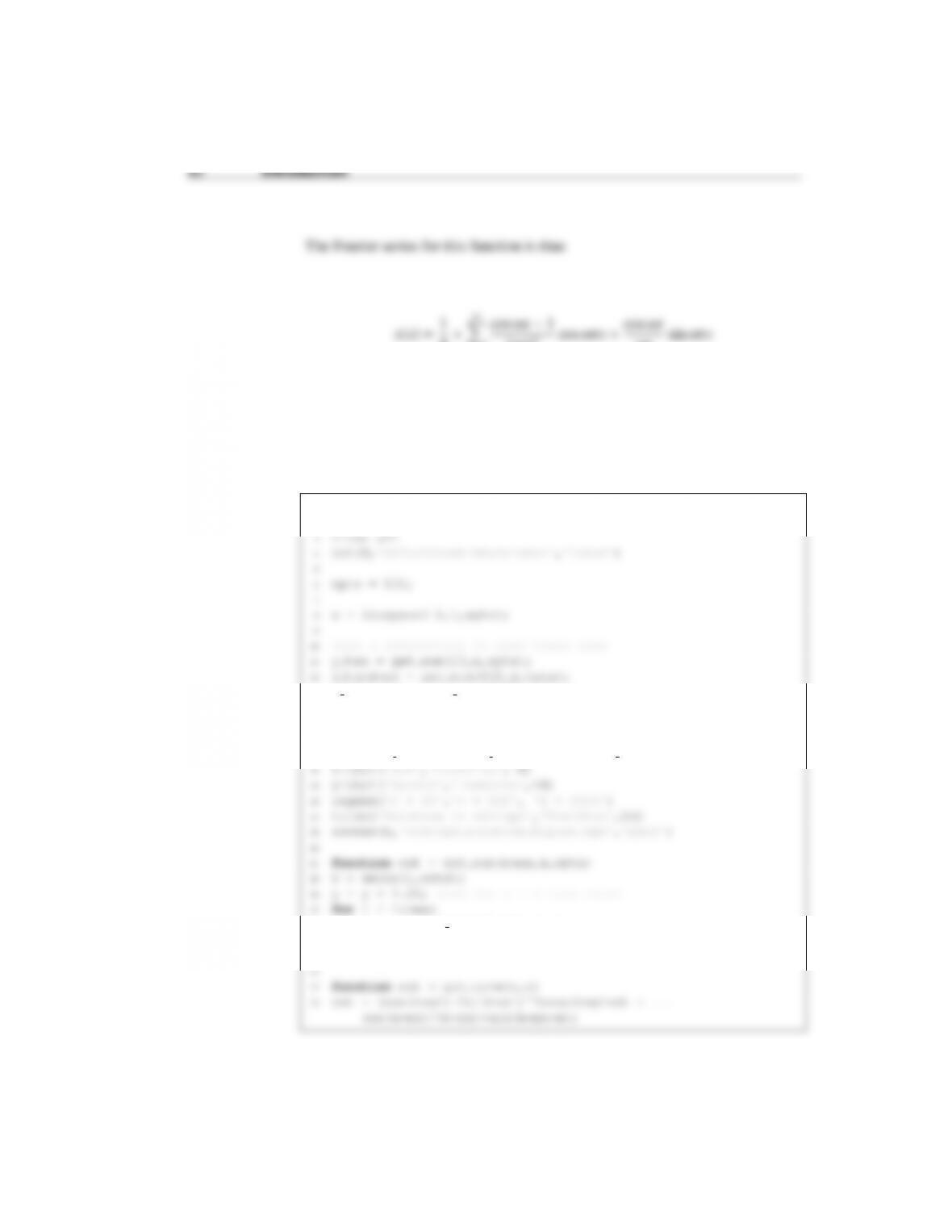
4+
n=1
(nπ)2cos nπx+cos nπ
nπsin nπx
(b) The Matlab program is:
1function s14c3p2
2clc
13 y thousand = get sum(1000,x,npts);
14
15 %make the plot
16 h = figure;
17 plot(x,y ten,‘-b’,x,y hundred,‘-k’,x,y thousand,‘-g’)
28 y = y + get term(i,x); %add one more term
29 end
30 out = y;
The output is
−1 −0.8 −0.6 −0.4 −0.2 0 0.2 0.4 0.6 0.8 1
−0.2
0
0.2
0.4
0.6
0.8
1
1.2
x
y(x)
Solution to s14c3p2
n = 10
n = 10 0
n = 10 0 0
(c) The Matlab program is:
11 %but easy to understand.
12 y exact = zeros(1,npts);
13 for i = 1:npts
14 if x(i) <0
15 y exact(i) = -x(i);
26 err k(j) = norm(y test–y exact);
28
29 %make the plot
30 h = figure;
42 Introduction
36 saveas(h,‘s14c3p3 solution figure.eps’,‘psc2’)
37
38 function out = get term(n,x)
39 out = (cos(n*pi)-1)/(n*pi)ˆ2*cos(n*pi*x) + …
cos(n*pi)/(n*pi)*sin(n*pi*x);
The output file is
100101102103
0.8
1
1.2
1.4
1.6
1.8
2
n
||y−y∗ ||
Solution to s14c3p3

2Linear equations
64 Linear equations
Problems
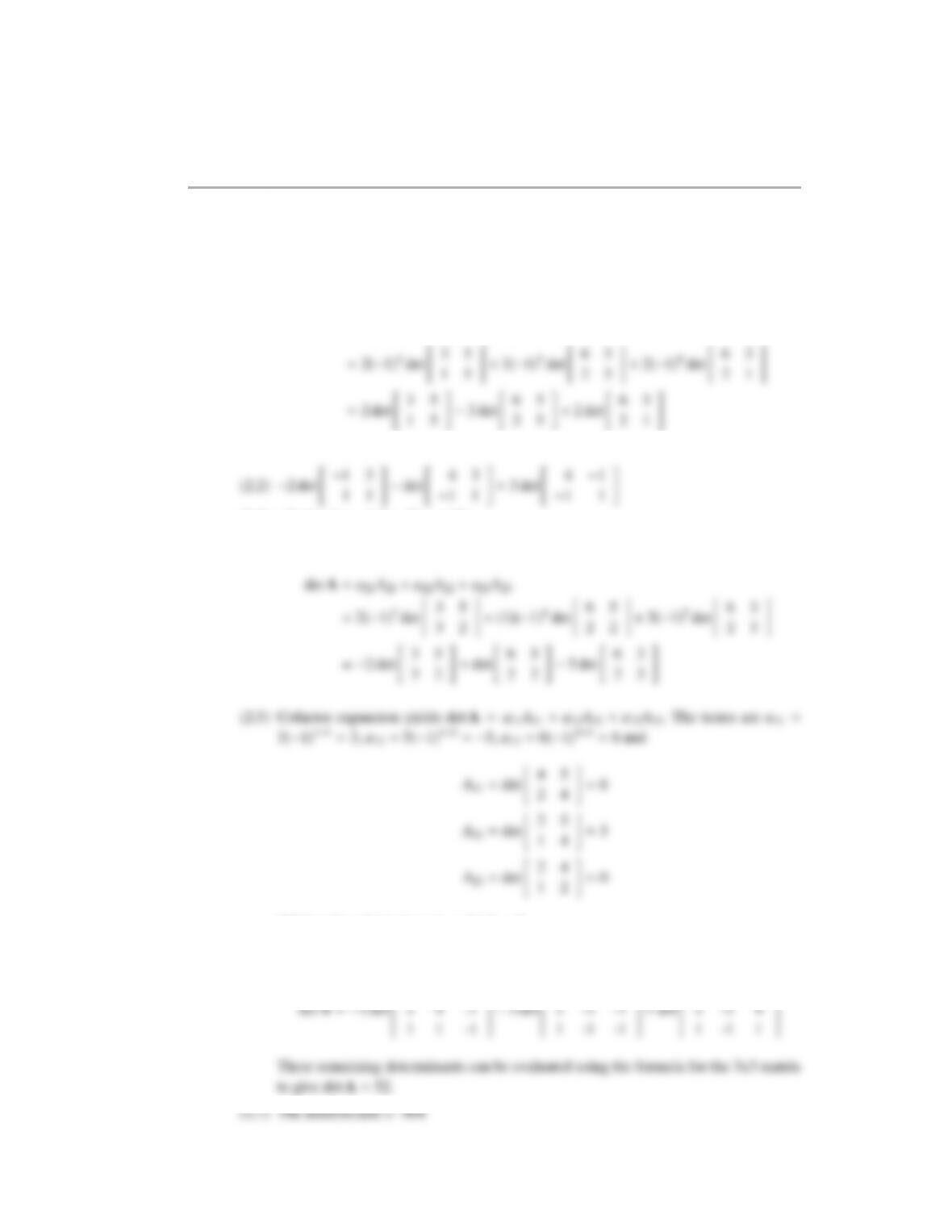
(2.1) The form of the co-factor expansion is
det A=a31A31 +a32A32 +a33 A33
(2.3) -10 (4 ×1× −1/4×10 =−10)
(2.4) Cofactor expansion yields
Making the substitution gives det A=3.
(2.6) The fastest choice is co-factor expansion on the 4th row:
6 -2 3
6 1 3
6 1 -2