4
6. The manipulation in the proof is similar to that in Theorem 6.4, so we only show the equivalence between the first
constraint and (6.65). In order to simplify the notation, we use ∆instead of ∆k. By applying Lemma 6.2, the inequality is
equivalent to
−Σ#¯
A+¯
D1∆¯
F$TΣ#¯
H+¯
D2∆¯
F$T
Σ#¯
A+¯
D1∆¯
F$−Σ0
¯
H+¯
D2∆¯
F0−I
=
−Σ¯
ATΣ¯
HT
∗−Σ0
∗∗−I
+
0
Σ¯
D1
¯
D2
∆
¯
FT
0
0
T
+
¯
FT
0
0
∆T
0
Σ¯
D1
¯
D2
T
≤0
By applying Lemma 6.3, the above holds if
−Σ¯
ATΣ¯
HT
Σ¯
A−Σ0
¯
H0−I
+
0
Σ¯
D1
¯
D2
Γ1
0
Σ¯
D1
¯
D2
T
+
¯
FT
0
0
Γ−1
2
¯
FT
0
0
T
≤0
−X+¯
FTΓ−1
2F−I+¯
FTΓ−1
2¯
FY
1ATX+HTKTATLT−HTJT0
∗−Y1+Y1¯
FTΓ−1
2¯
FY
1Y1ATY1ATY(LT−L
T)0
∗∗−X−I0XD1+KD2
<0(12)
Y>0,X−Y>0
which implies I−XY −1is invertible.
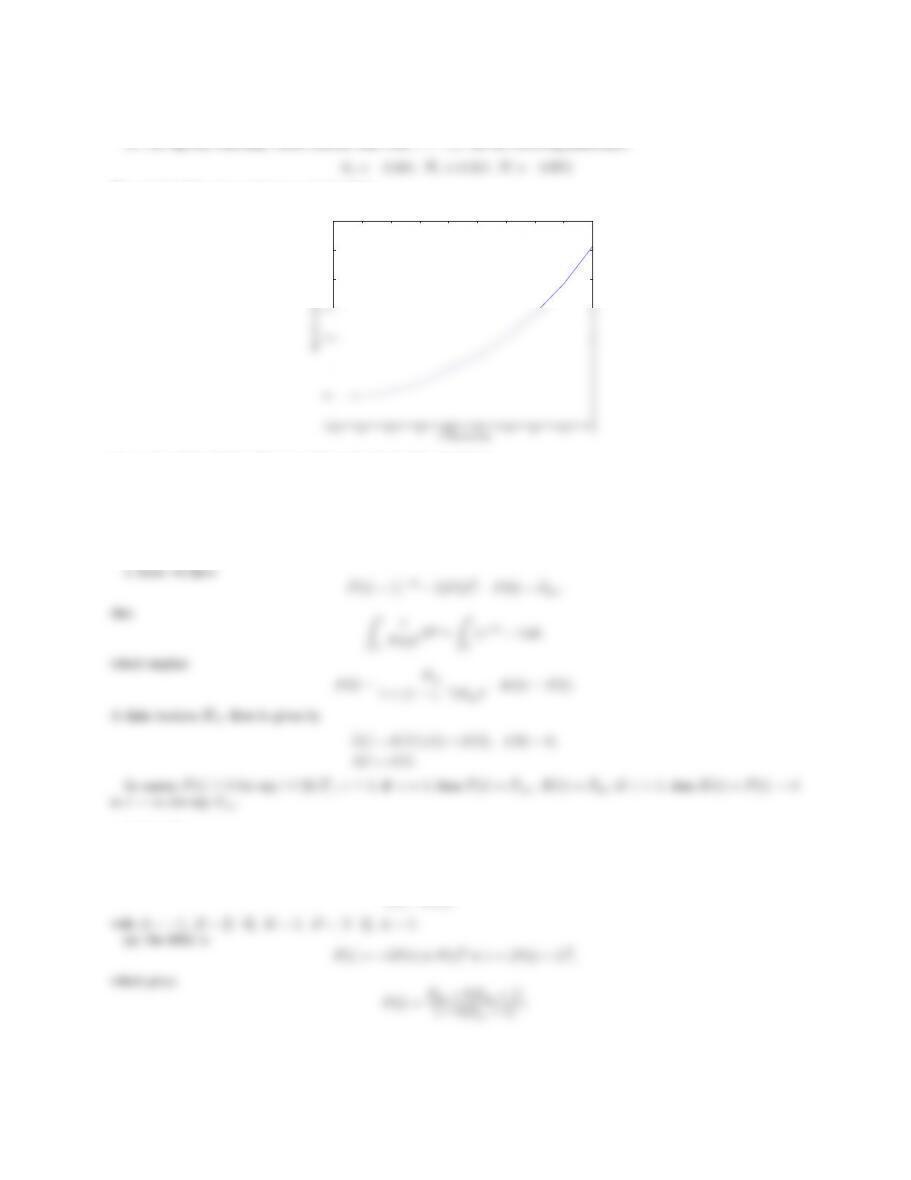
Ae=!00.00353835
00.0275018 “,H
e=%00.115262&,K=!0.0286107
0.218837 “,L=I, |δ|≥0.3.
5
−0.4 −0.3 −0.2 −0.1 0 0.1 0.2 0.
3
0
10
20
30
40
50
60
70
80
90
100
Uncertain Parameter
Filtering Error Variance
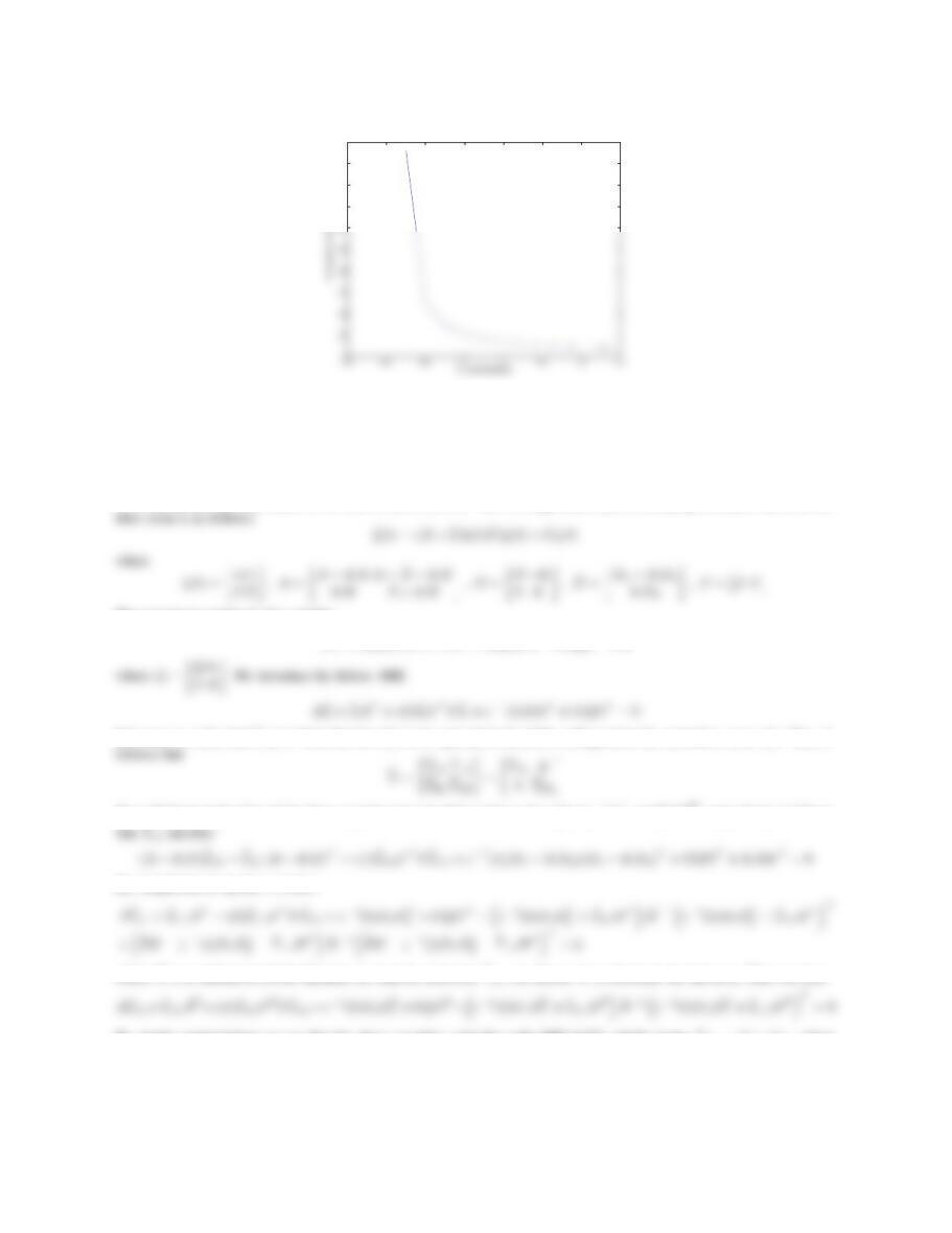
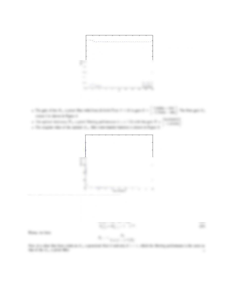
Fig. 2. Kalman filter error variance versus the uncertain parameter δ
Since the standard Kalman filter is less general than the filter form (6.7)-(6.8) or (6.48)-(6.49) with J=0, the Kalman filter
error variance is bigger than that of the optimal robust a priori filter.
9. We assume the state-space of the filter is (6.89)-(6.90). Then the augmented system including estimated state and the
filter error is as follows: ˙
ξ(t)=(¯
A+¯
D∆(t)¯
F)ξ(t)+ ¯
Gη(t)
where
A−KH
where ¯
Q=!Q0
0R“. We introduce the follow ARE
¯
A˜
Σ+˜
Σ¯
AT+ε(t)˜
Σ¯
FT¯
F˜
Σ+ε−1(t)¯
D¯
DT+¯
G¯
Q¯
GT=0
˜
Σ21 ˜
Σ22 “=!˜
0˜
Σ22 “
(A−KH)˜
Σ11 +˜
Σ11(A−KH)T+ε(t)˜
Σ11FTF˜
Σ11 +ε−1(t)(D1−KD2)(D1−KD2)T+GQGT+KRKT=0
By completion of squares, we have
+/˜
RK −ε−1(t)D1DT
2−˜
Σ11HT0˜
R−1/˜
RK −ε−1(t)D1DT
2−˜
Σ11HT0T
=0
By simply manipulations we see that the above equation coincides with ARE (6.92), which means ˜
Σ11 =P>Σ11, where
Σ11 is the (1,1) block of the matrix Σ. According to the definition of Σ, we see that Σ11 is the covariance of the filter error.
6
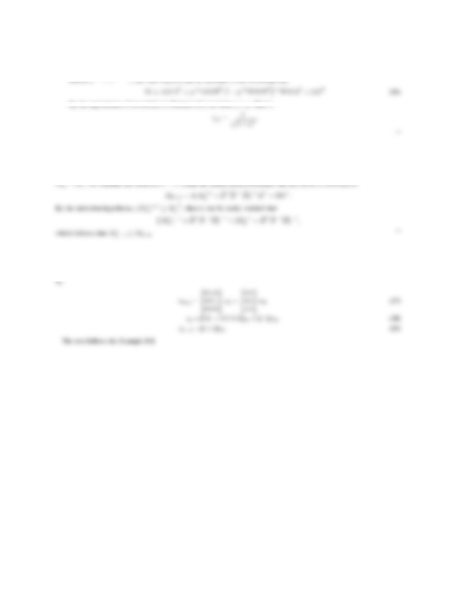
10. The optimal stationary robust Kalman filter with γ=1.21 has the following parameters:
Ae=−0.351,H
e=0.351,K=−0.973
The actually filter error variance is shown below.
0.05 0.1 0.15 0.2 0.25 0.3 0.35 0.4 0.45 0.
5
0.9
0.95
1
1.05
1.1
1.15
1.2
1.25
Uncertain Parameter
Filtering Error Variance
Fig. 3. The optimal stationary filter error variance versus the uncertain parameter δ
For the standard Kalman filter, we have
ˆx(t+1)=−ˆx(t)
ANSWERS TO EXERCISES OF CHAPTER 7
1. First, we have ˙
P(t)=(γ−2−1)P(t)2,P(0) = Px0,
thus 1t
1
z(t)=Hx(t)+D[wv]T
s(t)=Lx(t)
with A=−1,B=[1 0],H=1,D=[0 1],L=1.
(a) The DRE is ˙
P(t)=−2P(t)+P(t)2+1=(P(t)−1)2,
7
For 0<P
x0<1,P(t)is bounded and positive. An H∞filter is
˙
ˆx(t)=−ˆx(t)+K(t)(z(t)−ˆx(t)),ˆx(0) = 0,
ˆs(t)=ˆx(t),
To ensure nonnegative stabilizing solution, 2−γ−2>0, i.e., γ>1
√2.
For 1
√2<γ<1,Ps=1−√2−γ−2
γ−2−1, and As=−1+Ps(γ−2−1) = −22−γ−2, which is stable; for γ=1,Ps=1
2, which
is obviously a stable solution; for γ>1,Ps=1
˙p1=2p2+γ−2p2
2
˙p2=p3+γ−2p2p3
˙p3=1+γ−2p2
3
with the initial condition p1=p2=p3=0. Solving the differential equation above, together with 7.16, we obtain the finite
P(t)=1−(1 −2Px0)e−2t
2,
which is bounded and positive for any Px0. Thus, Px0can be any nonnegative value.
8
6. Set Z(t)=P2(t)−P1(t), then
˙
Z(t)=A[P2(t)−P1(t)] + [P2(t)−P1(t)]AT+P2(t)(γ−2LTL−HTH)P2(t)
−P1(t)(γ−2LTL−HTH)P1(t)
=!A+1
HI
⇔Rank !I−B
0I“!A−jwI B
HI
“=Rank !A−BH −jwI 0
HI
“=n+p
⇔The matrix A−BH has no purely imaginary eigenvalues.
‘G˜sw (s)‘<γ. It follows from Theorem 7.7, there exists a stabilizing solution P=PT≥0to the ARE:
(A−BH)P+P(A−BH)T−PHTHP +γ−2PL
TLP =0.(14)
By applying a state-space transformation we can have that
A21 A2“,P=!00
0P2“,H=[H1H2],L=[L1L2],
and P2>0, then the ARE (14) gives
Let X=P−1
2>0, hence
XA2+AT
2X−HT
2H2+γ−2LT
2L2=0,
10. For any given γ>0there exists an H∞stationary filter that achieves the H∞performance γ, if and only if there exists
P=PT>0and Ksuch that
(A−KH)P+P(A−KH)T+γ−2PL
TLP +BBT<0,
i.e.,
AP +PA
T+BBT−KHP −PHTKT+γ−2PL
TLP < 0.(15)
Choose Q=QT≥BBT,Q>0, then there always exist P=PT>0such that
9
since Ais stable. Further set K=1/2γ−2PHT, and the left hand side of inequality (15) becomes
AP +PA
T+BBT−KHP −PHTKT+γ−2PL
TLP
=AP +PA
T+BBT+γ−2P(LTL−HTH)P
≤AP +PA
T+Q+γ−2P(LTL−HTH)P
1 (a) By Theorem 8.3, the existence of an H∞a priori filter is equivalent to the existence of a solution Pk=PT
k>0,k =
0,1,··· ,N to the following DRE:
Pk+1 =(
1+Pk
Pk−γ−2)−1=Pk
1+(1−γ−2)Pk
,(16)
ˆx−
k+1 =ˆx−
k+P−
k
r+P−
k
(zk−ˆx−
k),
and the prediction error variance is computed by the DRE
P−
k+1 =P−
k
k
,P
−
0=Px0.
wk+1 =wk(17)
zk=φT
kwk+vk(18)
sk=wk(19)
10
0 2 4 6 8 10 12 14 16 18 2
0
−0.8
−0.7
−0.6
−0.5
−0.4
−0.3
−0.2
−0.1
0
0.1
0.2
k
Filter gains
K1,k
K2,k
•The gain of the H∞a priori filter with form (8.16-8.17) at N=20is gain K=!7.6856e−002
−7.7049e−001“. The filter gain Kk
versus kis shown in Figure 4.
•The optimal stationary H∞a priori filtering performance is γ=1.53 with the gain K=!0.0708372
−1.01048 “.
01234567891
0
0
50
Frequency(rad/sec)
Fig. 5. The singular value plots of the optimal H
∞filter error transfer function
4. Proof:
By Theorem 8.6, the existence of an H∞a posteriori filter is equivalent to the existence of a solution Pk=PT
k>0to the
DRE:
Mk+1 =Pk,P
0=Px0(22)
P−1
k+1 =M−1
k+1 +1−γ−2.(23)
Hence, we have
kis shown in Figure 6.

11
0 2 4 6 8 10 12 14 16 18 2
0
−0.1
0
0.1
0.2
0.3
0.4
0.5
0.6
0.7
0.8
k
Filter gains
K1,k
K2,k
•The optimal stationary H∞a priori filtering performance is γ=1.00 with the gain K=!0.96406
−0.086011“.
•The singular value of the optimal H∞filter error transfer function is shown in Figure 7.
0 50 100 150 200 250 30
0
0
0.2
0.4
0.6
0.8
1
1.2
1.4
Frequency(rad/sec)
Singular value
Fig. 7. The singular value plots of the optimal H
∞filter error transfer function
•Ais a (not strict) stable matrix, hence γinf −→ 1.
6. Proof:
By Theorem 8.8, the stationary H∞a posteriori filtering problem is solvable if and only if there exists a stabilizing solution
M=MT>0to the ARE:
AMAT−M−AM ¯
HT(¯
R+¯
HM ¯
HT)−1¯
HMAT+GGT=0.
Since H=L, the ARE is rewritten as
M=AMAT−AM HT[(1 −γ−2)−1I+HMHT]−1HMAT+GGT(24)
12
(2) Stable A
Define η−2=γ−2−1, the ARE Eq.(24) can be rewritten in the following way:
M=AMAT+η−2AM HT[I−η−2HMHT]−1HMAT+GGT(26)
By the equivalence of (a) and (c) in Theorem 8.2, we have η>µ. That is,
γinf =µ
21+µ2.
7. The optimal H∞a priori and a posteriori filtering performances are 1.97 and 1.00 respectively. The Kalman filter can be
obtained by setting γ→∞. Hence we get the Kalman a posterior filter and a priori filter provide H∞filtering performances
of 1.42 and 3.44, respectively.
8. Proof : By the initial condition M′
0>M
0, the result holds for k=0. Assuming that it holds up to k, k ≥0, i.e.,
M′
k≥Mk. We consider the result for k+1. Using the matrix inversion lemma, the Eq. (8.53) is rewritten as
Mk+1 =A[M−1
k+¯
HT¯
R−1¯
H]−1AT+GGT.
By the induction hypothesis, (M′
k)−1≤M−1
k, then it can be easily verified that
10. Define xk=[sk−3sk−2sk−1]T,wk=[skvk]T, a state space representation of the model and the measurement is given
by
xk+1 =
010
001
xk+
00
00
wk(27)