Chapter 10
Answers to Review Problems
Finance For Executives – 4th Edition
1. Historical returns.
a.
If one accepts that stocks are riskier than corporate bonds, which are riskier than government
bonds, which are riskier than Treasury bills, then the annual data does not appear to support a
naïve understanding of theory. In 2000, 2001, 2002, and in 2005, the returns on stocks were less
than the returns on corporate bonds. In 1994, 1996, 2001, and in 2006, Treasury bills yielded a
b.
These apparent anomalies can be explained mainly by changes in long-term interest rates, the
slope of the yield curve, or changes in the risk perception by the market for corporate bonds.
When market interest rates rise, bond values will fall resulting in lower returns. The opposite will
c.
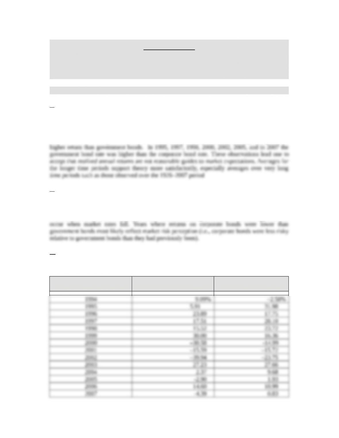
The market risk premium for each of the periods observed can be found in the table below.
Time Period
Market Risk Premium
versus Government Bonds
Market Risk Premium
versus Treasury Bills
10-1
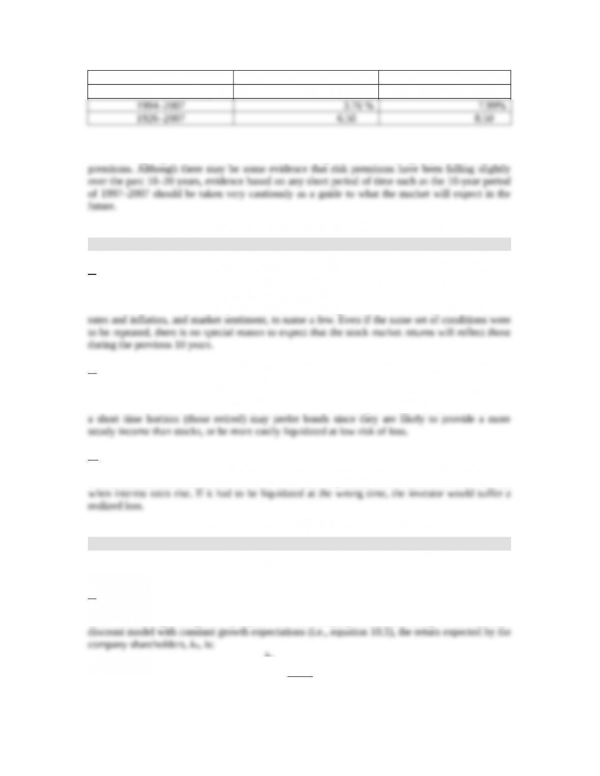
Annual arithmetic averages
One can conclude that risk premiums for individual years are highly volatile. Negative premiums
for assuming higher risk do not make sense as a guide for estimating expected future risk
2. Risk and return.
a.
The statement is dangerous although it could be true since the future is unknown. Future returns
on the market will be affected by several factors such as growth of the economy, level of interest
b.
Investors will hold bonds or stocks depending on their tolerance to risk, their need to be assured
of a steady income, their time horizon, and their current consumption requirement. Investors with
c.
This is false as can be seen from the table of returns in question 1. The value of a bond will fall
3. The cost of equity and the cost of debt.
Both statements are false.
a.
The statement ignores growth prospects for the company stock. According to the dividend
kE
g
P
DIV
0
1
10-2
where DIV1 is the dividend next year, P0 is the current share price, and g is the expected growth
b.
The interest expenses represent the cost of financial liabilities such as debt to banks or bonds.
Liabilities of any company include these debts but also other liabilities such as accounts payable
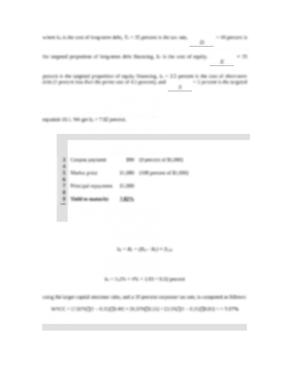
4. The cost of debt.
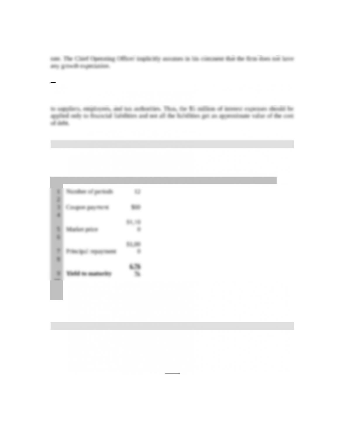
The current market price of the bond is $1,100 (110 percent of $1,000 par value). Using a
spreadsheet as it is shown in the text to solve equation 10.1, we get kD = 6.76 percent.
A B C D E F G
10
11 The formula in cell B9 is: =RATE(B1,B3,-B5,B7).
12
5. The cost of equity.
According to the dividend discount model with constant growth expectations (i.e., equation 10.5)
the return expected by the company shareholders, kE, is:
kE
g
P
DIV
0
1
10-3
where DIV1 = $2.10 is the dividend expected for next year [$2.00 × (1 + 0.05) = $2.10, where
kE
percent2.9092.005.00420.005.0
50$
10.2$
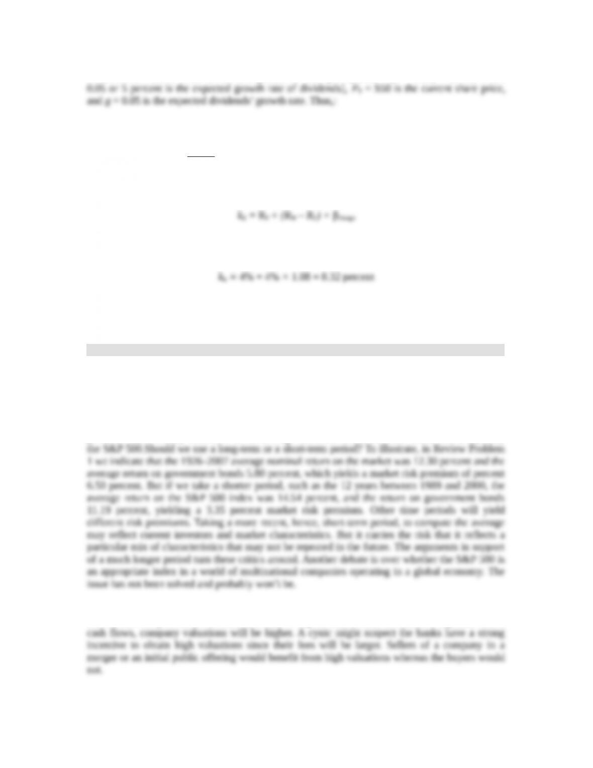
According to the capital asset pricing model (i.e., equation 10.11):
where RF = 4 percent is the risk-free rate, RM – RF = 4 percent is the market risk premium, and
βOgono = 1.08 is Ogono’s equity beta coefficient. Thus,:
The average of the two values for kE, 8.8 percent, should be the best estimate of the cost of equity
for Onogo Inc.
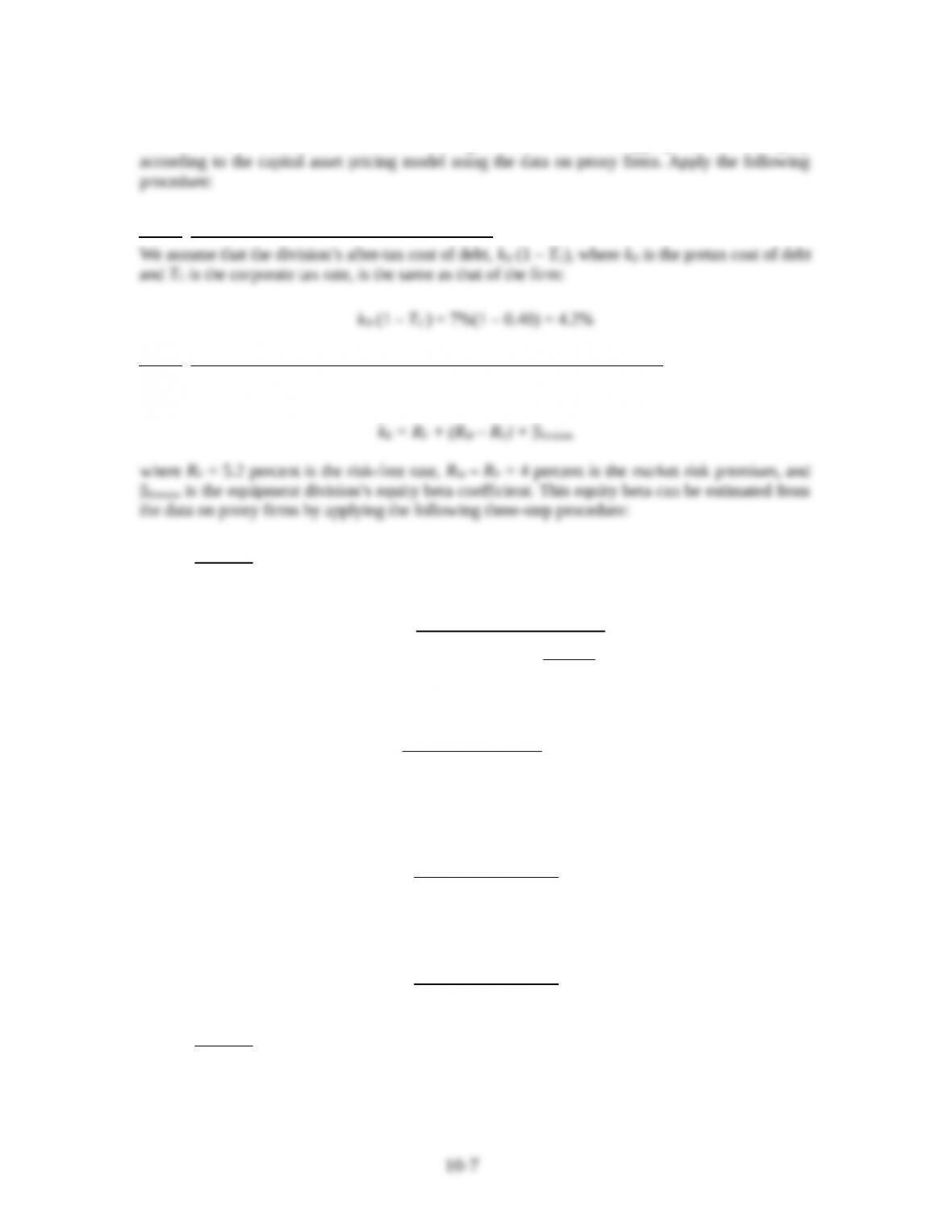
6. Practical application of the capital asset pricing model.
This question is about some of the practical problems encountered in applying the capital asset
pricing model (CAPM). Of the variables in the model, RF (the risk-free rate) is directly observable
and (the firm’s equity beta) can be fairly easily measured by regressing the returns of a
particular security, or securities belonging to the same industrial sector, on the returns of a market
index. It is the expected average return on the market, RM, which creates the measurement
problem. RM is usually estimated as the average historical return on some broad index, typically
Why have some investment banks been using very low market risk premiums? Since the lower
the market risk premium, the lower the cost of capital that is used to discount expected future
10-4
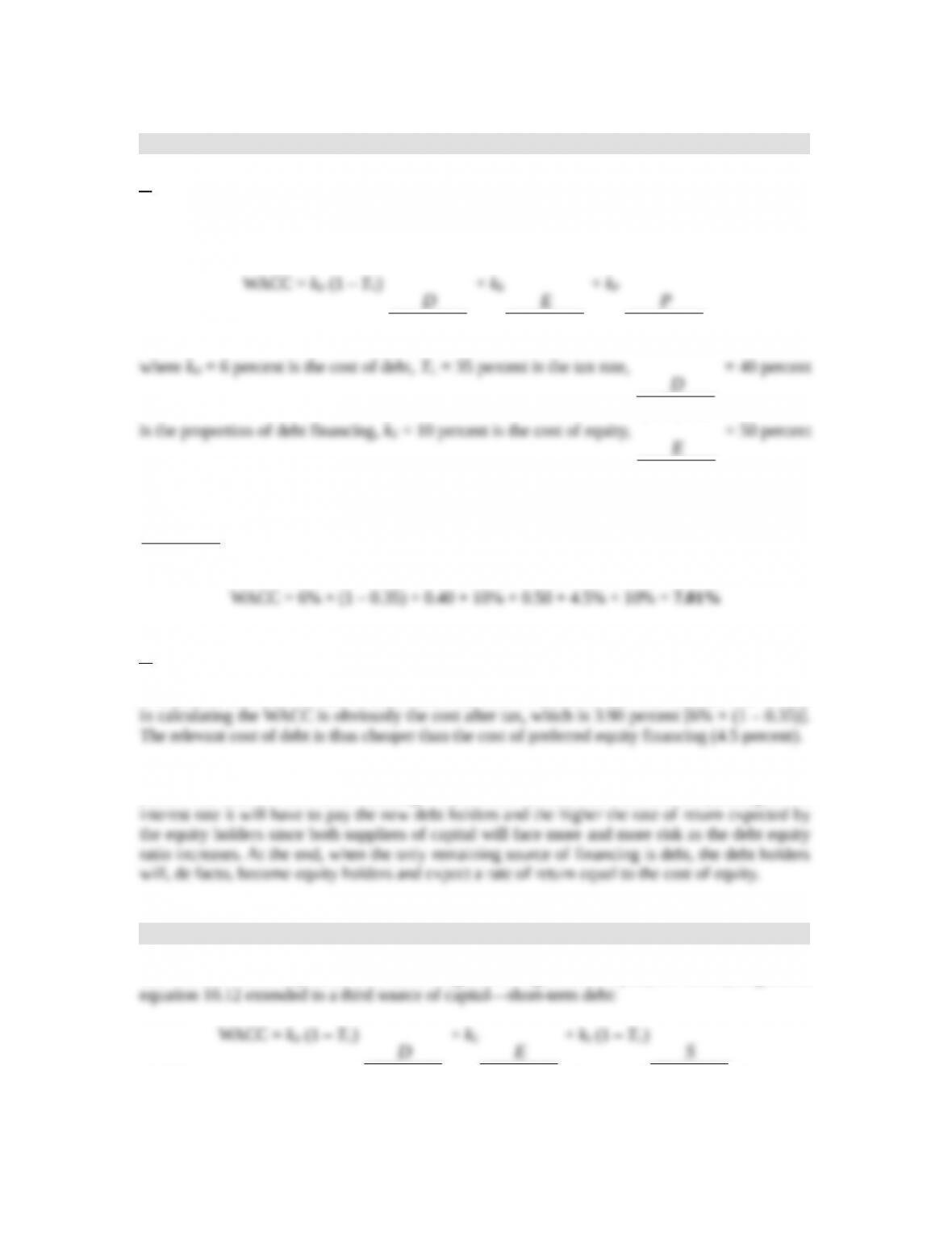
7. Calculating the weighted average cost of capital (WACC).
a.
According to equation 10.12 extended to a third source of capital—preferred stock—Tale’s cost
of capital, or weighted average cost of capital (WACC) is:
To estimate the equipment division’s weighted average cost of capital, you need to estimate its
after-tax cost of debt and its relevant financing ratios as well as its appropriate cost of equity
Step 1: Estimate the division’s after-tax cost of debt.
Step 2: Estimate the division’s cost of equity based on data from proxy firms.
According to the capital asset pricing model (see equation 10.11), we have:
Step 2.1: Estimate the asset betas of the proxy firms using equation 10.7.
Equity
Debt
)rateTax1(1
equity
asset
For proxy A:
44.0
00.1)40.01(1
70.0
asset
For proxy B:
68.0
80.0)40.01(1
00.1
asset
For proxy C:
72.0
70.0)40.01(1
02.1
asset
Step 2.2: Estimate the equipment division’s asset beta as the average of the proxies’ asset
betas
10-7
61.0
3
72.068.044.0
asset
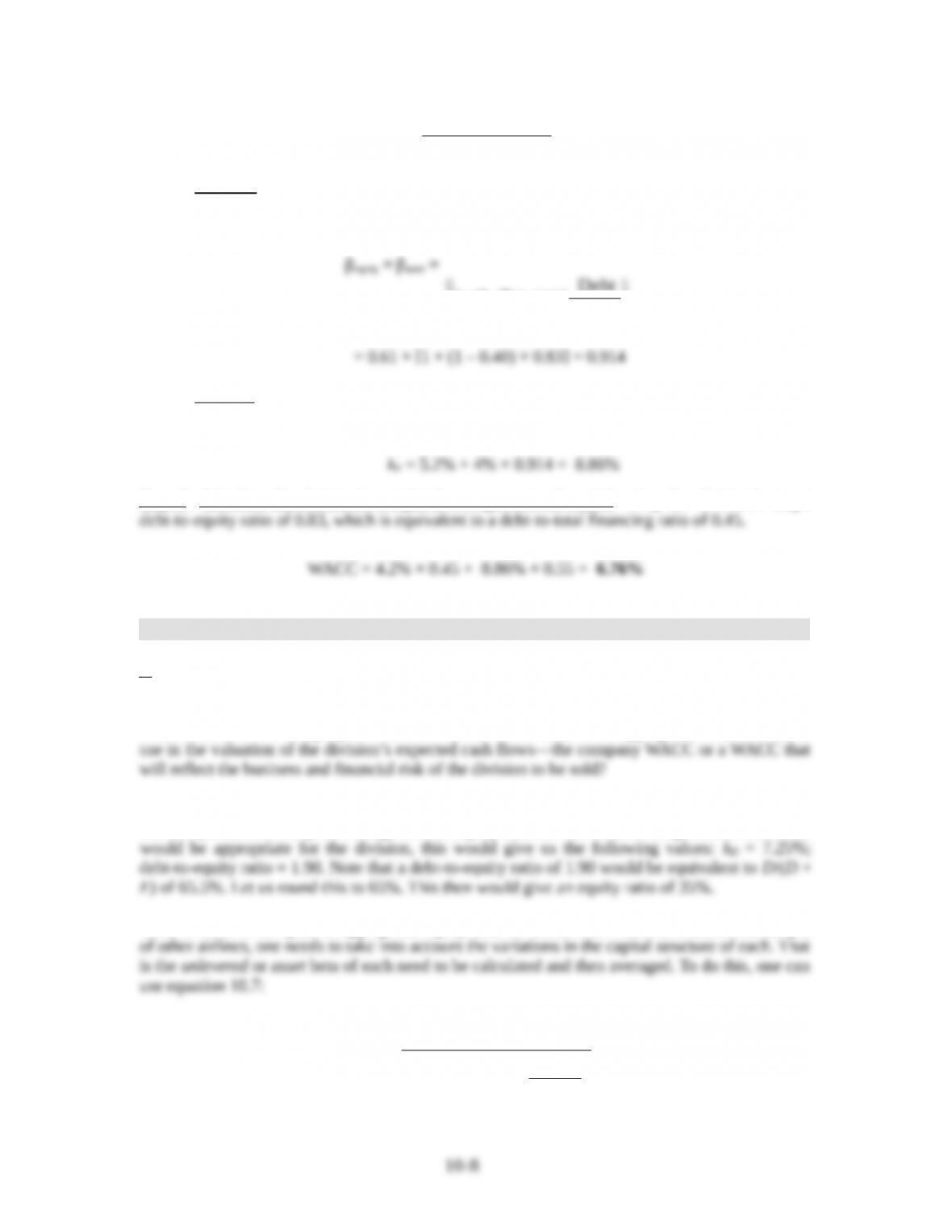
Step 2.3: Estimate the equipment division’s equity beta by relevering the division’s
estimated asset beta of 0.70 at the division’s target debt-to-equity ratio of 0.83, using
equation 10.6.
Equity
Debt
)rateTax1(1
= 0.61 × [1 + (1 – 0.40) × 0.83] = 0.914
Step 2.4: Estimate the division’s cost of equity using its estimated equity beta of 1.344
and the capital asset pricing model.
Step 3: Calculate the division’s weighted average cost of capital using the division’s target
10. Estimation of cost of capital for a spinoff.
a.
The CEO wants to have an estimate of the value of a division that is to be sold before beginning
discussions with the company’s investment bankers. The issue is the appropriate discount rate to
To calculate the division’s WACC, both the cost of debt and equity will need to be estimated. If
one accepts that the sample’s average debt-to-equity ratio as well as the average cost of their debt
Next, in order to compute an appropriate equity beta for the division from the betas of the sample
Equity
Debt
)rateTax1(1
β
β
equity
asset
10-8
where the tax rate is 30% and D/E is the debt-to-equity ratio for each airline at market valuations.
This formula would give A = 0.64, B = 0.41, C = 0.69, D = 0.66, and E = 0.46. If we can
Equity
Debt
rate)Tax(11ββ
assetequity
which gives:
Divison’s equity = 1.33
The cost of equity of the division, given by the capital asset pricing model (equation 10.11), is:
where RF = 5 percent is the risk-free rate, RM – RF = 4 percent is the market risk premium, and
βDivision = 1.33 is the division’s equity beta coefficient.
and the division cost of capital is:
b.
If the company’s WACC had been used to discount the division’s cash flow, this would have
10-9