Chapter 2 Diffusion in dilute solutions page 2-1
Chapter 2 Diffusion in dilute solutions
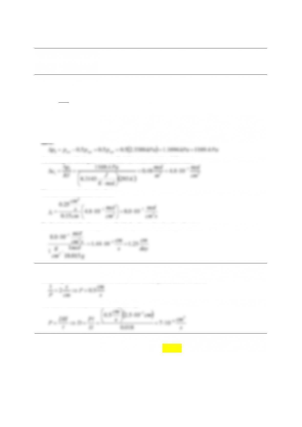
1. Water evaporation
To find the rate of evaporation, we need to find the flux of water across the air film:
11 c
DH
jΔ= l
Since the film is made up of air, H = 1. We are given D and ℓ, so we need to find Δc1. We first
calculate the difference in the partial pressure of water across the film. From a steam table we
find that at 20 °C, psat = 2.3388 kPa. Since the air immediately above the water is saturated we
1
Assuming an ideal gas, we can find the concentration difference:
()
3
7
3
1
1108.448.0
2933145.8
4.1169
cm
mol
m
mol
K
molK
J
Pa
RT
p
⎟
⎠
⎞
⎜
⎝
⎛
⋅
Δ
We can now calculate the flux:
scm
mol
cm
mol
cm
s
cm
j2
7
3
7
2
1100.8108.4
15.0
25.0 −− ⋅=
⎟
⎠
⎞
⎜
⎝
⎛⋅=
To find the height change, we divide by the molar density of water:
cm
s
cm
g
mol
cm
g
scm
mol
015.18
1
1
100.8 5
3
2
7
⋅
⋅−
−
2. Diffusion across a monolayer
Recalling that the resistance is the inverse of the permeance, we have:
s
cm
P
cm
s
P5.02
1=⇒=
We know that the permeance is given by:
()
cm
cm
s
cm
P
DH
2
6
7
105.25.0
−
−
⋅
⎟
⎠
⎞
⎜
⎝
⎛
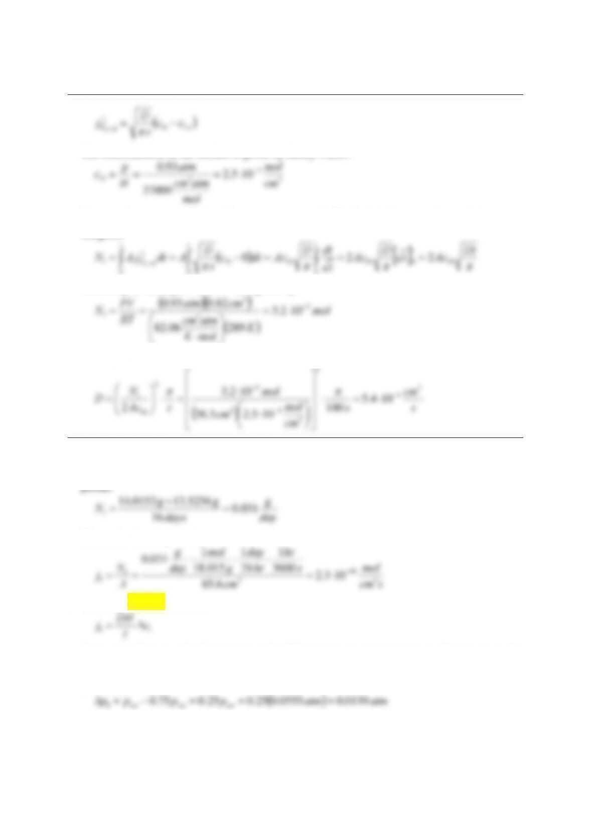
3. Diffusion coefficient of NO2 in water
We treat the water as a semiinfinite slab. From Eq. (2.3-18) we know that the flux at the surface
is given by:
Chapter 2 Diffusion in dilute solutions page 2-2
∞
=−= 110
0
1cc
t
D
π
The concentration at the surface is given by Henry’s Law:
5
3
10 105.2
37000
93.0
cm
mol
mo
l
atmcm
atm
H
p
Since we have a semiinfinite slab we assume c1∞ = 0. To find the flux over the total time t, we
integrate:
ππππ
Dt
D
t
dtD
t
D
ttt
0
0
00
Assuming an ideal gas, the flux N1 is given by:
()
()
()
K
molK
atmcm
cmatm
RT
PV
3
3
1102.3
28906.82
82.093.0 −
⎟
⎟
⎠
⎞
⎜
⎜
⎝
⎛
⋅
Solving for D, we have:
()
s
cm
s
cm
mol
cm
mol
tAc
N
2
6
2
3
52
5
2
10
1104.5
180
105.23.36
102.3
2
−
−
−
⎥
⎥
⎥
⎦
⎤
⎢
⎢
⎢
⎣
⎡
⎟
⎠
⎞
⎜
⎝
⎛⋅
⋅
⎟
⎠
⎞
⎜
⎝
⎛
ππ
4. Permeability of water across a polymer film
The rate of water loss can be found by linear regression or by simply using the first and last data
days
16
1=
The molar flux is given by:
mol
cm
s
hr
hr
day
g
mol
day
g
A
N
10
2
1
1103.2
6.85
3600
1
24
1
015.18
1
031.0
−
⋅⋅⋅
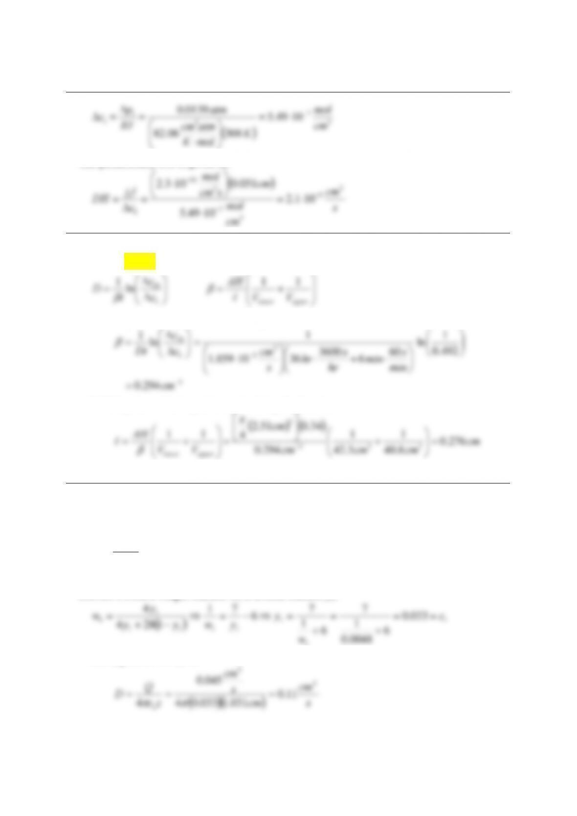
From Eq. (2-2.10) we have:
DH
We need to find Δc1. We first calculate the difference in the partial pressure of water across the
film. From a steam table we find that at 35 °C, psat = 0.0555 atm. Since the air inside the bag is
saturated, we have:
1
Assuming an ideal gas, the concentration difference is:
Chapter 2 Diffusion in dilute solutions page 2-3
()
3
7
3
1
11049.5
30806.82
0139.0
cm
mol
K
molK
atmcm
atm
RT
p
⎟
⎟
⎠
⎞
⎜
⎜
⎝
⎛
⋅
Δ
The permeability DH is given by:
()
s
cm
cm
mol
cm
scm
mol
c
j
2
5
3
7
2
10
1
1101.2
1049.5
051.0103.2
−
−
−
⋅
⎟
⎠
⎞
⎜
⎝
⎛⋅
Δ
5. Diaphragm cell
From Ex. (2.2-4) we have:
⎠
⎞
⎜
⎝
⎛+=
⎟
⎠
⎞
⎜
⎝
⎛
Δ
Δ
upperlower VV
AH
c
c
t
1
1
10
l
β
(a) Using the first equation and solving for β we have:
⎞
⎛
Δ
10
1
c
1
⎞
⎛
1
(b) Using the second equation and solving for ℓ we have:
()()
cmcmcm
cm
VV
AH
upperlower
8.40
1
3.42
1
294.0
34.051.2
4
11
332
2
⎟
⎠
⎞
⎜
⎝
⎛+
⎥
⎦
⎤
⎢
⎣
⎡
⎟
⎠
⎞
⎜
⎝
⎛+= −
π
β
(c) Since the porosity is the same, the result is the same.
6. Measuring diffusion coefficient of gases
The maximum concentration will be at the center of the pipe so r = 0 and the equation reduces
to:
Dz
Q
c
π
4
1=
Dimensional analysis tells us that the concentration must be dimensionless, so we simply
convert it from a weight fraction w1 to a mole fraction y1:
()
1
1
1
1111
1
1033.0
6
0048.0
1
7
6
1
7
71
1284
4c
w
ywyy
y
+
+
−+
Solving for D, we have:
()( )
s
cm
cm
s
cm
zc
Q
2
3
1
031.1033.04
045.0
4===
ππ
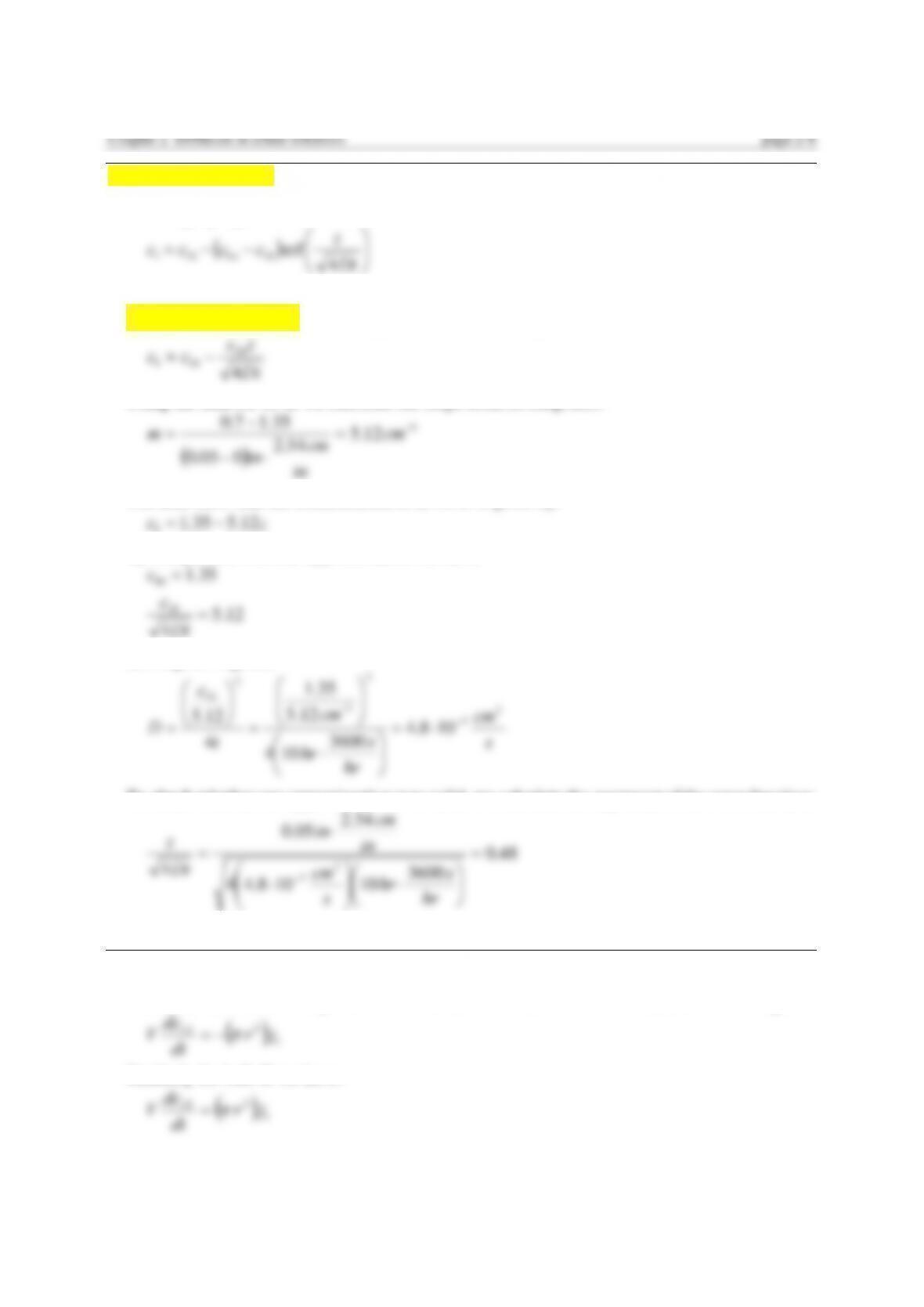
7. Carburizing of steel
Rearranging Eq. (2.3-15) we have:
⎠
⎞
⎝
⎛
z
Since this is a semiinfinite slab, c1∞ = 0. Assuming the argument of the error function is small
(i.e. less than about 0.7), we can approximate it as the argument itself:
zc
10
Using the data for 10 hr we calculate the slope from its endpoints:
()
1
54.2
005.0
35.17.0 −
⋅−
−
in
cm
in
The data show that the concentration c1 at 10 hr is given by:
1−=
By comparison with our approximation we have:
4
35.1
10
10
=
=
Dt
c
Solving for D gives:
cm
hr
s
hr
cm
t
c
2
7
2
1
2
10
3600
104
12.5
35.1
4
12.5 −
−
⎟
⎠
⎞
⎜
⎝
⎛⋅
⎟
⎟
⎠
⎞
⎜
⎜
⎝
⎛
⎟
⎠
⎞
⎜
⎝
⎛
To check whether our approximation was valid, we calculate the argument of the error function:
48.0
3600
10108.44
54.2
05.0
42
7
=
⎟
⎠
⎞
⎜
⎝
⎛⋅
⎟
⎟
⎠
⎞
⎜
⎜
⎝
⎛⋅
⋅
=
−
hr
s
hr
s
cm
in
cm
in
Dt
z
The assumption is valid.
8. Twin-bulb method
We define the direction of positive flux is from bulb A into bulb B. A balance on bulb A gives:
1
2
1jr
dt
dc
Similarly for bulb B we have:
1
2
1jr
dt
dc
Chapter 2 Diffusion in dilute solutions page 2-5
Subtracting the second equation from the first, we get:
1
2
11 2jrcc
dt
d
The flux is given by:
BA cc
DH
In this case H = 1 since there is no interface. Combining these equations and substituting Δc1 for
c1A – c1B we have:
dt
V
Dr
c
cdrcD
dt
cd
Vll
2
1
1
2
11 2
2
π
π
−=
Δ
⇒
Δ
−=
Δ
Integration gives:
V
tDr
t
c
c
ecc
V
tDr
c
c
dt
V
Dr
c
cd l
ll
2
1
10
2
101
2
10
1
0
2
1
12
ln
2
π
ππ
−
Δ
Δ
Δ=Δ⇒−=
⎟
⎟
⎠
⎞
⎜
⎜
⎝
⎛
Δ
Δ
⇒−=
Δ
Δ∫∫
9. Steady-state flux out of a pipe with porous wall
From Eq. (2.4-29) we have:
⎟
⎠
⎞
⎜
⎝
⎛
∂
∂
∂
∂
=
∂
∂
r
c
r
rr
D
t
c11
Since we are at steady state, the time derivative is zero and we are left with:
00 11 =
⎟
⎠
⎞
⎜
⎝
⎛
⇒
⎟
⎠
⎞
⎜
⎝
⎛
=dr
dc
r
dr
d
dr
dc
r
dr
d
r
D
Integrating twice we have:
r
dr
11
This is subject to boundary conditions:
0
1
==
==
cRr
ccRr ii
Applying the second and then the first we have:
0
01
0
0
1
0
00
ln
ln
ln
ln
lnln0
R
R
Rc
RAB
R
R
c
R
R
RABBRA
i
i
i
ii
−=−=
−=⇒+=
Substitution gives:
Chapter 2 Diffusion in dilute solutions page 2-6
0
0
ln
ln
ln
ln
ln
R
R
R
r
R
R
Rc
R
R
rc
i
i
o
i
The flux at the outside of the pipe is given by Fick’s Law:
i
i
Rr
i
i
Rr
R
R
R
Dc
R
R
r
Dc
dr
dc
Dj
0
0
1
0
1
1
lnln
0
0
=−=−=
=
=
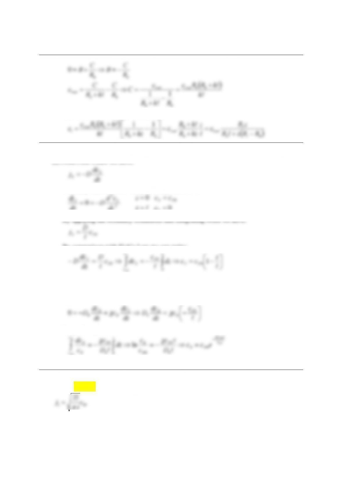
10. Controlled release of pheromones
From a balance on the device we have:
1Ajr
dt
dc
Since we are interested in the steady state case, the time derivative is 0 and we find that the rate
of sublimation must equal the rate of transport through the membrane. Substituting for r0 and j1
⎦
⎣
⎠
⎝
s
mol
(a) Solving for c1 we have:
s
mol
s
mol
17
17
106
106
−
−
⋅
⋅
(b) Solving for r0 or Aj1 gives:
()
s
mol
cm
mol
cm
s
cm
cm
ADH
3
8
2
122
11 108.4104.8
06.0
1092.18.1
−−
−
⎠
⎞
⎝
⎛⋅
⎟
⎟
⎠
⎞
⎜
⎜
⎝
⎛⋅
11. Measuring age of antique glass
Based on Example 2.3-3, we have:
()
∞
=−
+
0
1
1cc
t
KD
π
Since the water is consumed as it enters the glass, we assume that c1∞ = 0. The total hydration is
Chapter 2 Diffusion in dilute solutions page 2-7
then:
()
(
)
ππ
KDt
t
dtKD
tt
+
+
1
110
00
Solving for t we have:
()
⎟
⎠
⎞
⎜
⎝
⎛
+
10
1
21 Ac
N
KD
π
12. Diffusion in a reactive barrier membrane
(a) Mass balances on mobile species 1 and immobile species 2 give:
2
11
12
2
212
∂∂
=−
∂∂
∂=−
∂
R
R
cc
Dkcc
tz
ckcc
t
(b) The boundary conditions for this situation are:
1220
2
1
00
<==
∂
∂
tallzc cc
c
(c) The reaction term would exist only in a front, moving across the film with time. Everywhere
else in the film either c1 or c2 is zero and the reaction term drops out of the differential
equations.
13. Diffusion of dopant in arsenide
From Eq. (2.4-14) we have:
z
Dt
AM
1
2
4
/−
π
Since the maximum concentration will be at z = 0 i.e. the site of the scratch we can write:
z
c
c
Dt
AM
max1
1
max1
2
4
/−
π
Solving for t, we have:
()
()
⎟
⎟
⎠
⎞
⎜
⎜
⎝
⎛
⋅
⎟
⎟
⎠
⎞
⎜
⎜
⎝
⎛
−
−
s
cm
cm
c
c
D
z
10ln104
104
ln4 2
11
2
4
1
max1
2
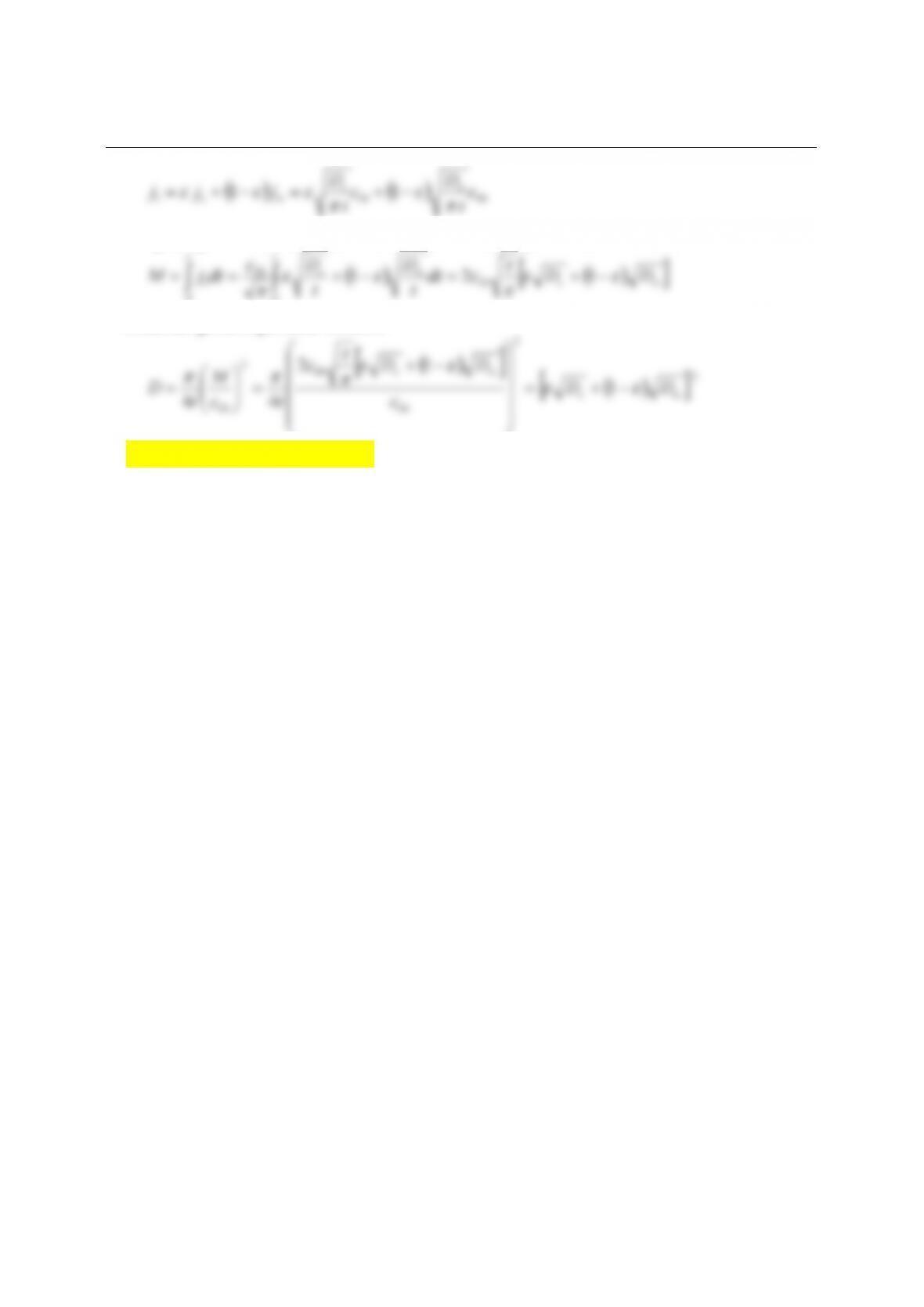
14. Concentration profile in Fick’s experiment
(a) For the cylinder, the cross sectional area A is constant. Since the experiment is at steady
state, j1 is also constant. Using Fick’s Law, we have:
Chapter 2 Diffusion in dilute solutions page 2-8
D
dz
The boundary conditions are:
sat
cz
11
100
==
The first boundary condition tells us that C = 0. Applying the second gives:
Dc
D
B
sat
1
(b) For the funnel, the cross sectional area A is not constant. The area at height z is given by:
2
⎠
⎝
l
where k has been defined for convenience. Since the area is a function of z, the condition
of steady state requires that the product Aj1 be constant. As a result we have:
()
dz
dj
dz
dA
dz
Ajd 1
1
1
Using Fick’s Law to substitute for j1 and the above expression for A we have:
⎤
⎡−+++
⎤
⎡−= 21
2
2
120 dz
cd
dc
21
0
dz
We now define a function u and redefine our differentials in terms of it:
2
1
2
2
2
2
1
2
22
2
111
0
du
cd
k
dz
du
du
cd
dz
cd
du
dc
dz
du
du
dc
dz
dc
kzRu
=
⎟
⎠
⎞
⎜
⎝
⎛
=
+=
Our equation now becomes:
2
1
2
2
2
1
2
2
1
2=+⇒+= du
dc
du
cd
du
cd
du
dc
This equation is of the Euler-Cauchy form, which means the solution is of the form
The solution is a linear combination of the two roots:
kzR
C
B
u
C
Bc +
+=+=
0
1
Applying the same boundary conditions as above we find:
Chapter 2 Diffusion in dilute solutions page 2-9
l
l
lk
RkR
C
R
kR
c
R
C
B
R
C
B
satsat
sat
=
−
+
=⇒−
+
=
−=⇒+=
001
00
1
00
1
00
11
0
The concentration profile is therefore:
() ()
00
1
0
0
1
00
001
1
11
RRzR
zR
c
z
kzR
kR
c
RkzRk
kRRc
csatsat
sat
−+
=
+
+
=
⎥
⎦
⎤
⎢
⎣
⎡−
+
+
=
l
l
ll
l
l
l
15. Bacteria between membranes
(a) From Fick’s Law we have:
dc
At steady state we know that jS is independent of z:
2
00
=
=
ccz
By comparison with Fick’s Law we can write:
⎠
⎞
⎝
⎛−=⇒−=⇒=− ∫∫ lll
z
c
D
dz
dc
z
S
c
c
SS
S
S
S
0
0
0
0
0
(b) Once again assuming steady state, we know that jB is independent of z. We also know
from the boundary conditions that jB = 0 at z = 0 and z = ℓ, so jB = 0 for all z. The given
equation then becomes:
⎠
⎞
⎝
⎛−=⇒+−= l
0
00
B
B
S
B
Bc
dz
dc
dz
dc
dz
dc
Integration gives:
ll
0
0
0
0
0
0
000
0ln D
zc
BB
S
z
B
B
c
c
S
B
B
S
B
B
D
zc
c
c
D
c
c
dc
χ
χχ
−
where cB0 is the concentration of B at z = 0.
16. Extraction of sucrose
From Eq. (2-3.18) the flux through the surface of a slice is:
t
D
π
The total flux is a weighted average of the individual fluxes:
Chapter 2 Diffusion in dilute solutions page 2-10
10101 11 c
t
D
t
D
wc
π
π
Integrating over time to get the total sucrose extracted per unit area we have:
t
wc
t
t
t
D
t
Dc
π
π
0
0
10
From the given expression we have:
2
10
10
44 wc
c
tc
t
⎟
⎟
⎠
⎜
⎜
⎝
⎟
⎠
⎜
⎝
Not sure this answers the question