Answers to Problems at the End of Chapter 6 6-16
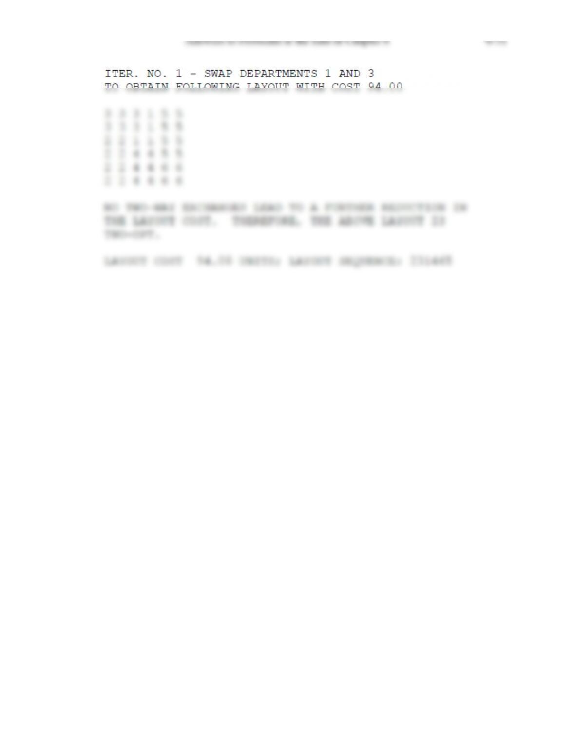
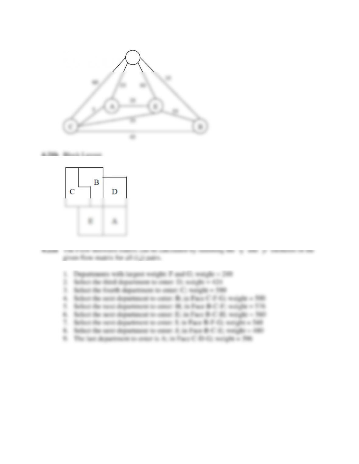
Adjacency Graph
Block Layout
6.19 1. Departments with largest weight: A and B; weight = 9
E
C
A
B
D
450
0
250
0
250
350
350
400
400
Answers to Problems at the End of Chapter 6 6-17
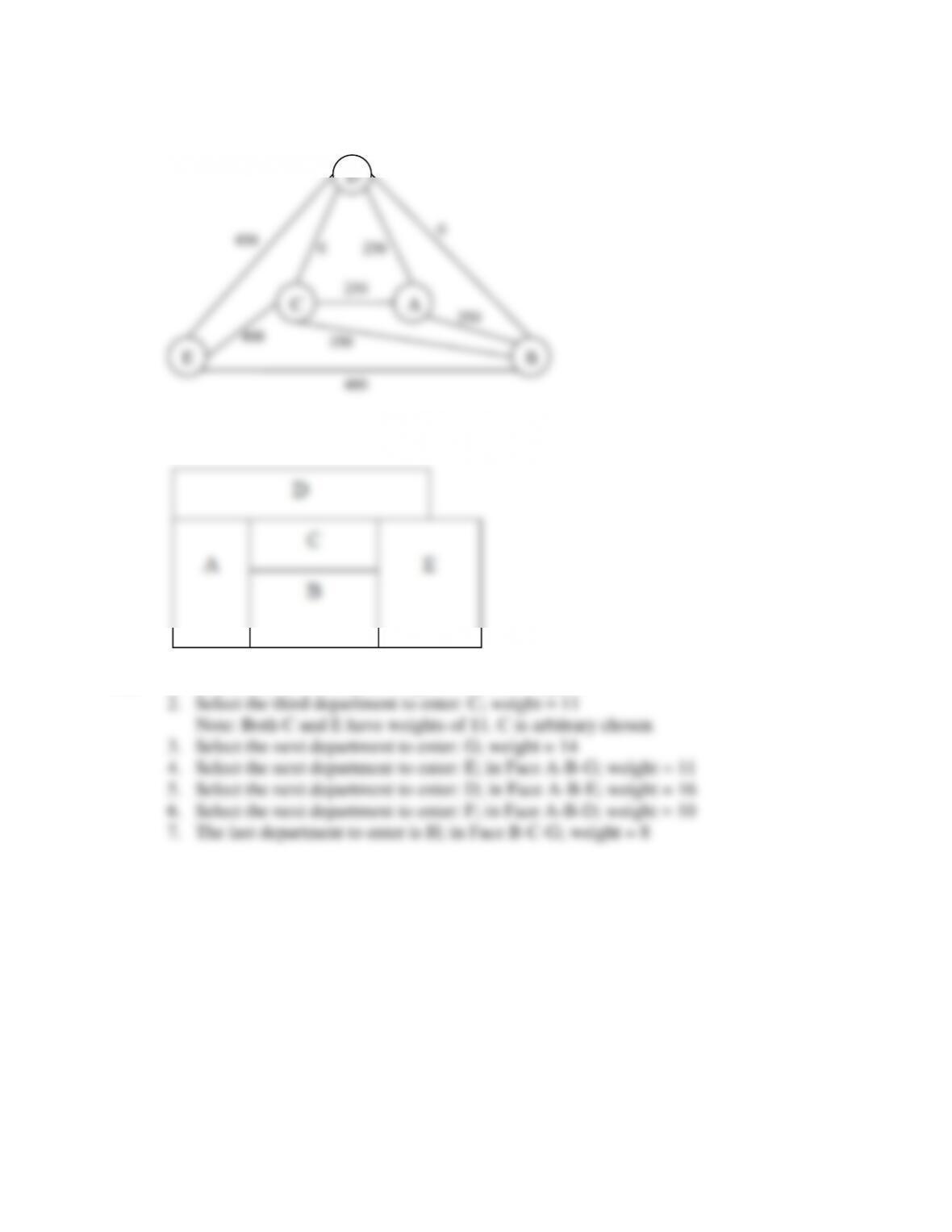
Adjacency Graph
Block Layout
6.20 1. Departments with largest weight: B and C; weight = 504
A
F
B
D
E
G
C
H
9
5
0
0
8
5
5
9
6
7
0
0
0
1
7
8
4
6
Answers to Problems at the End of Chapter 6 6-18
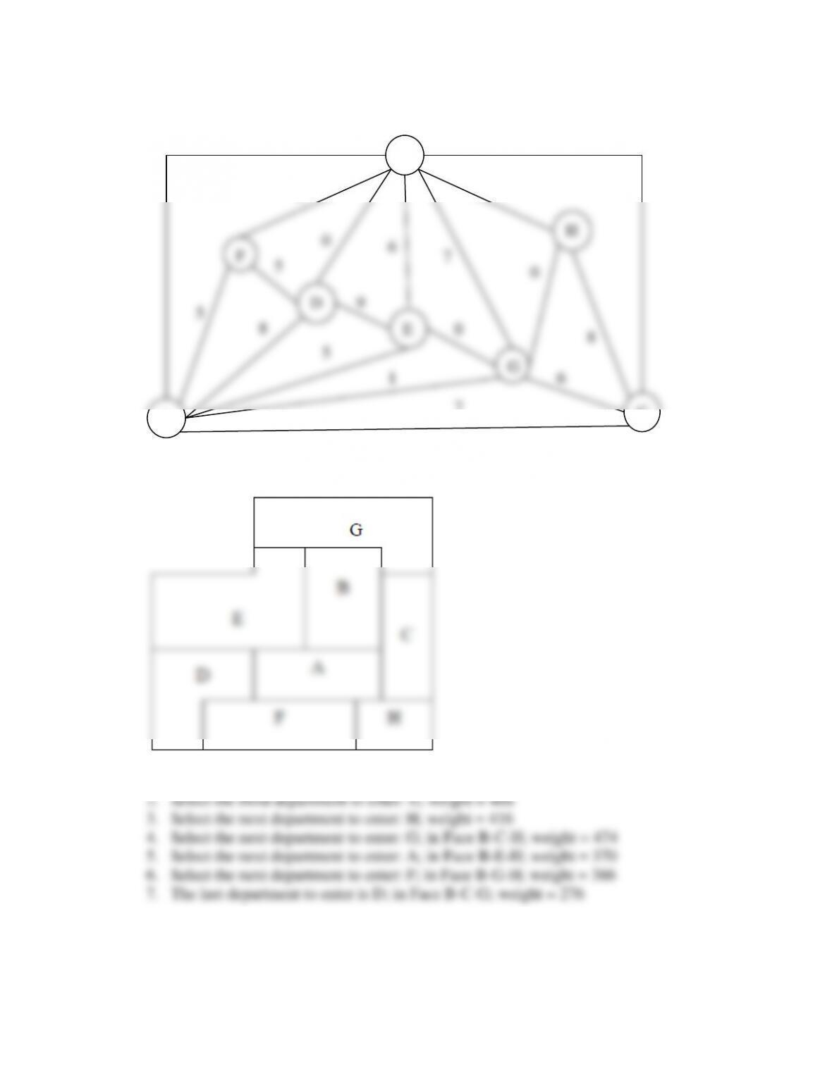
Adjacency Graph
Block Layout
C
D
B
G
F
H
E
A
504
76
0
282
122
188
94
20
68
24
136
302
56
352
180
296
40
154
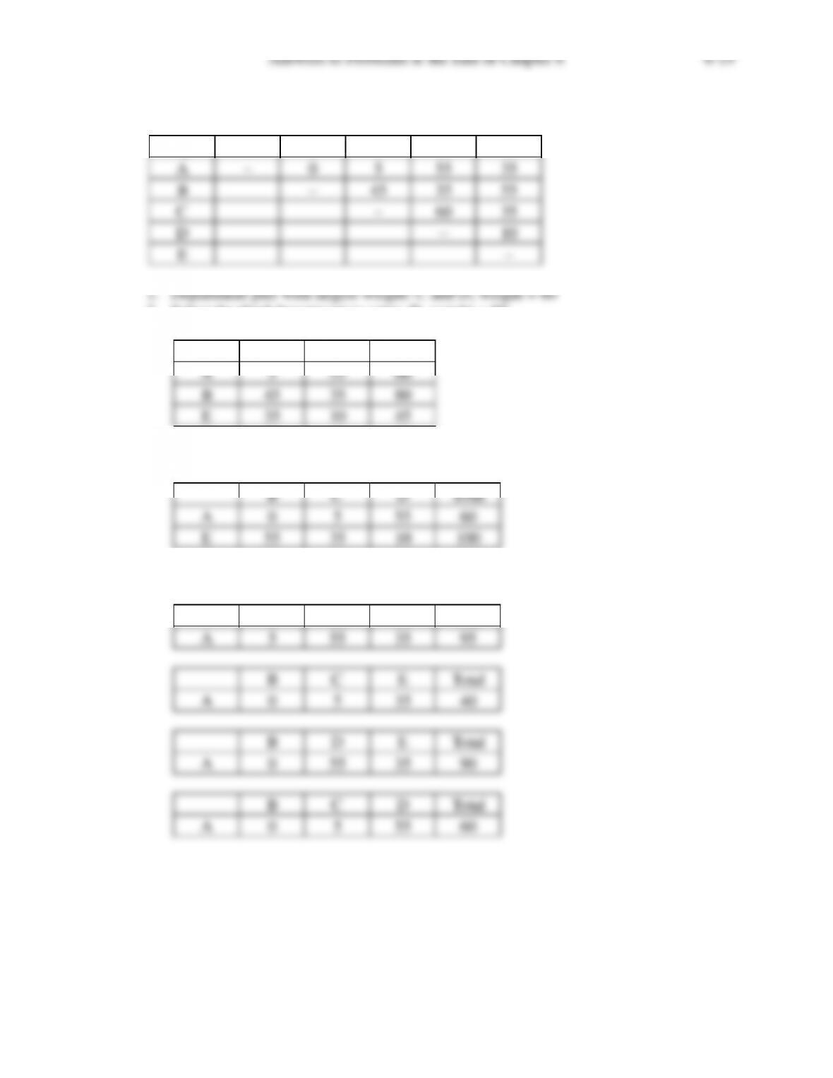
6.21a Flow-Between Chart
2. Select the third department to enter: B; weight = 80
3. Select the next department to enter: E; weight = 100
4. Department A enters the face C-D-E; weight = 95
A 0 55 35 90
Dept. A B C D E
A–0 5 55 35
B–45 35 55
C–60 35
D–10
E–
C D Total
A 5 55 60
B45 35 80
E35 10 45
B C D Total
A 0 5 55 60
E55 35 10 100
C D E Total
A 5 55 35 95
Answers to Problems at the End of Chapter 6 6-20
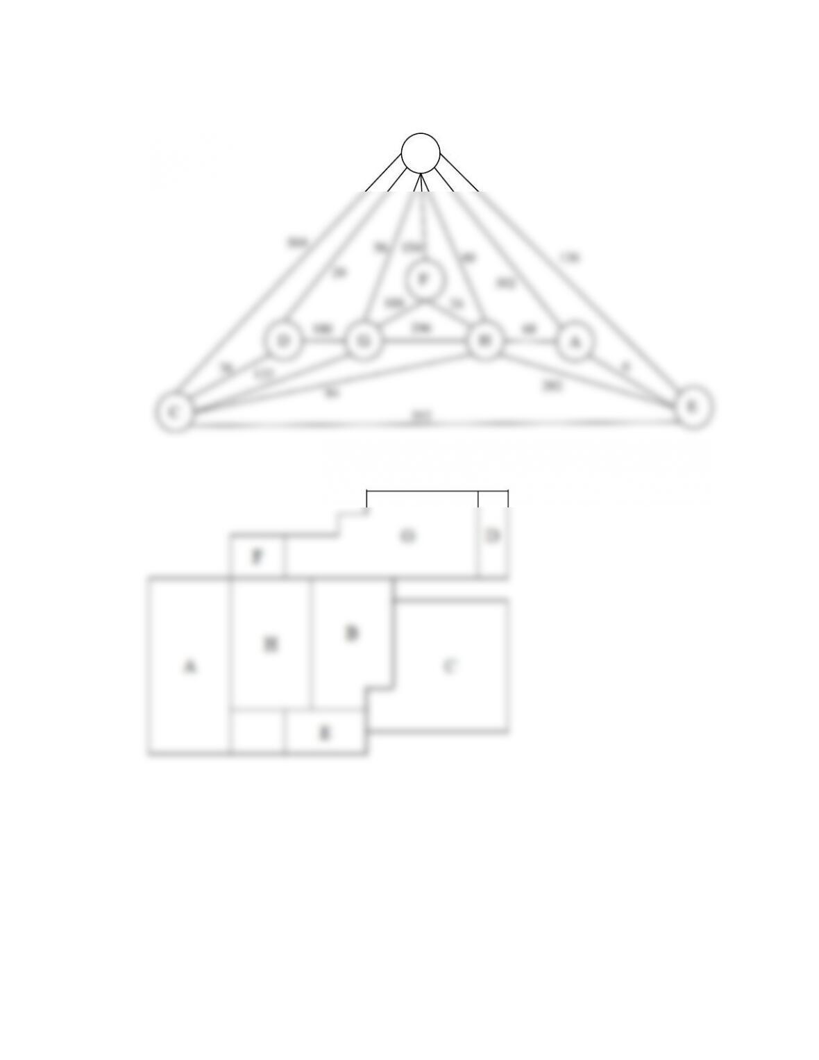
Adjacency Graph
6.21b Block Layout
C
A
E
B
D
60
55
35
35
10
55
35
5
45
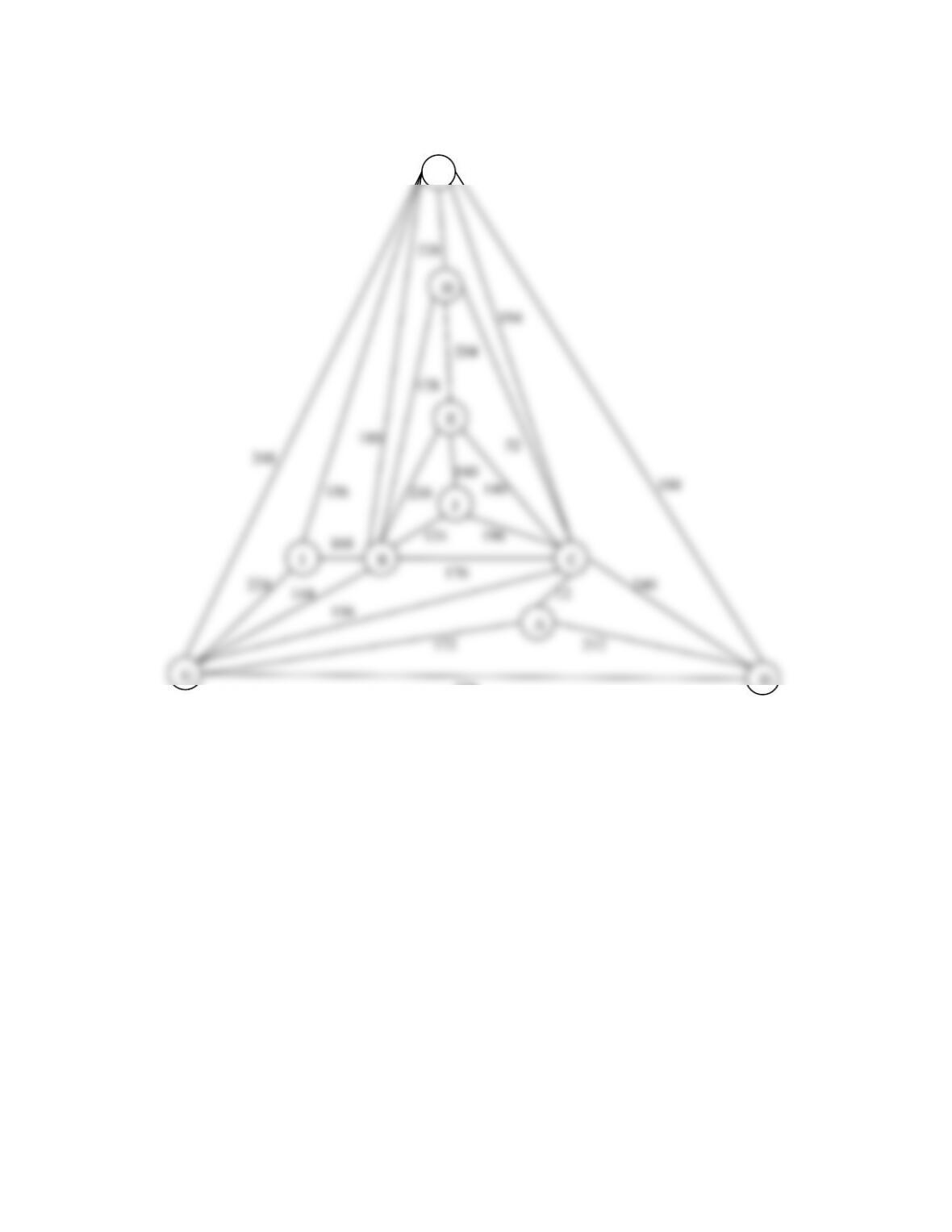
Answers to Problems at the End of Chapter 6 6-21
Adjacency Graph
A
B
C
D
E
F
G
H
I
J
248
224
156
180
188
240
156
172
212
144
236
168
176
124
196
216
140
128
32
160
184
204
228
12
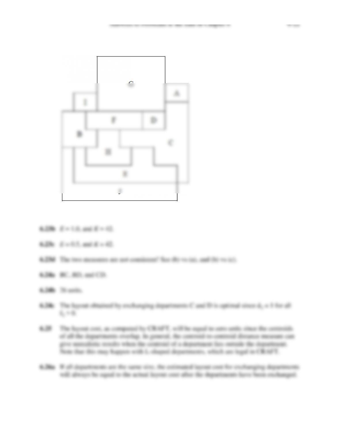
6.22b Block Layout
6.23a E = 1.0, and K = 28.
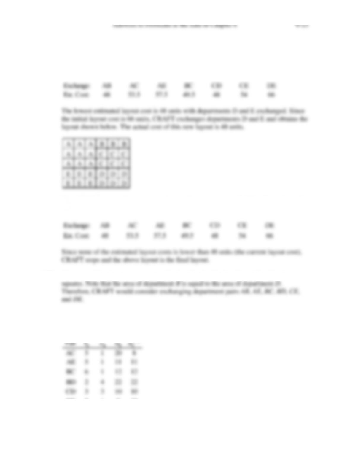
6.26b The initial layout cost is 93 units, and the estimated layout cost of exchanging B and C is
75 units; however, the actual layout cost after B and C have been exchanged is 111 units.
6.27 The following estimated layout costs are computed for the initial layout:
Next, CRAFT repeats the same procedure as above to compute the following estimated
layout costs:
6.28a The areas of the departments are A = 48 , B = 40 , C = 85, D = 40, and E = 62 unit
6.28b Let dij be the distance between departments i and j in the current layout; let 𝑑𝑖𝑗
𝐴𝐸 be the
estimated distance between departments i and j if departments A and E are exchanged.
Given the flow and cost data, we have:
Exchange: AB AC AE BC CD CE DE
Est. Cost: 48 53.5 57.5 49.5 48 54 66
Pair
fij cij dij dij
AE
AC 5 1 20 8
AE 5 1 11 11
BC 6 1 12 12
BD 2 4 22 22
CD 3 3 10 10
Answers to Problems at the End of Chapter 6 6-24
6.29a The areas (in unit squares) of the departments are A = 4, B = 8, C = 6 , D = 6 , E = 8 , and
6.29d In general, given the same problem data, we would expect MULTIPLE to obtain a lower
layout cost than CRAFT since MULTIPLE considers a larger set of (2-way) department
6.30a Principal weaknesses of CRAFT: 1. no control over department shapes; 2. only adjacent
6.30b True. Both CRAFT and NEWCRAFT are “path dependent” heuristics. Since the two
6.31
6.32b The distance matrix for the given layout is computed as follows:
6.32c False. BLOCPLAN uses three bands; if two non-adjacent or unequal-area departments
6.32d Advantages: A rectangular shape is often the preferred shape for a department; also, with
6.33 To avoid unrealistic department shapes, we set Ri equal to two for all the departments.
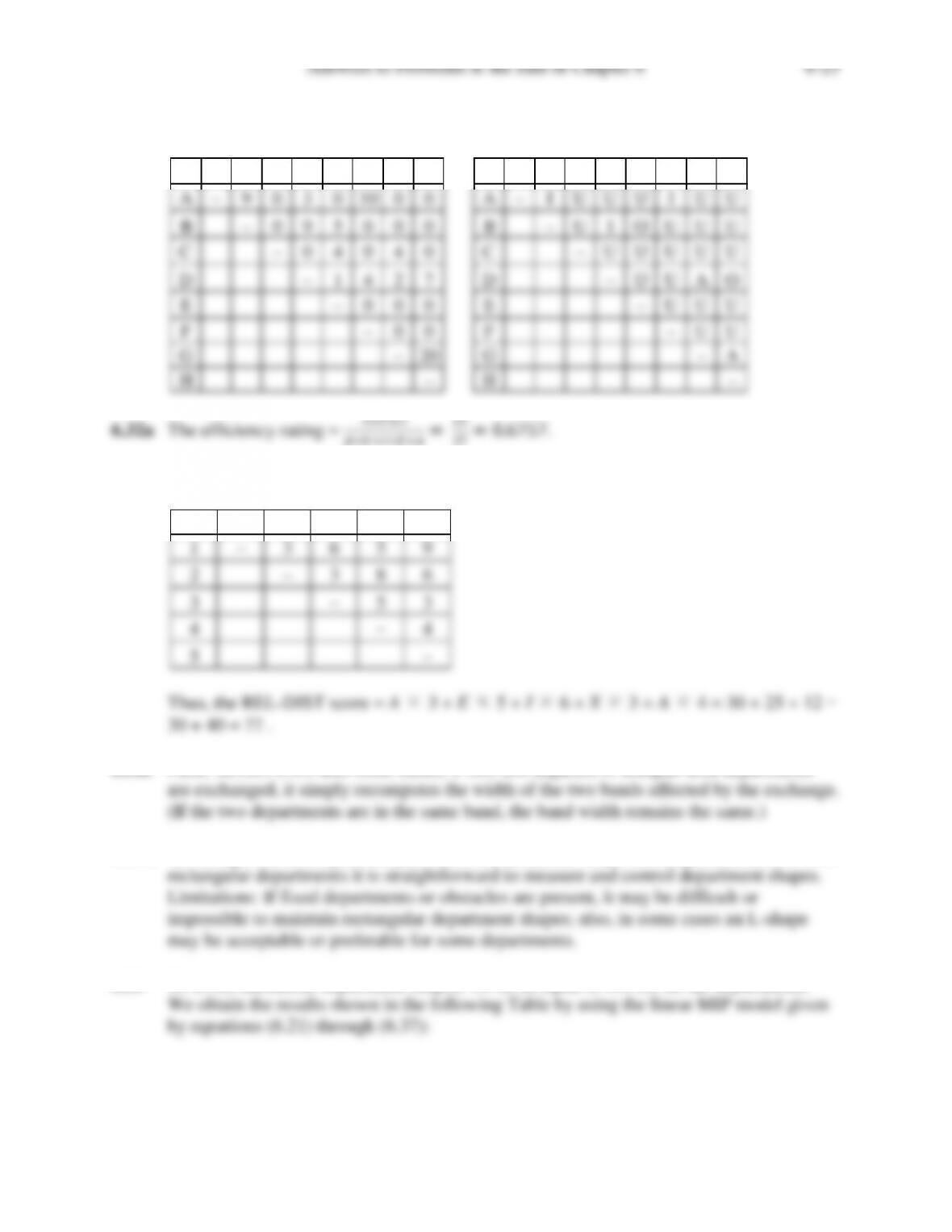
Flow–Between Chart Relattionship Chart
A B C D E F G H A B C D E F G H
A–9 0 3 0 10 0 0 A –I U U U I U U
B–0 9 5 0 0 0 B –U I O U U U
C–0 4 0 4 0 C –U U U U U
D–1 4 2 7 D –U U A O
E–0 0 0 E –U U U
F–0 0 F –U U
G–20 G–A
H–H–
Dept. 1 2 3 4 5
1–3 6 5 9
2–3 8 6
3–5 3
4–4
5–
Answers to Problems at the End of Chapter 6 6-26
The objective value we obtained from the model is 14,929.74 units.
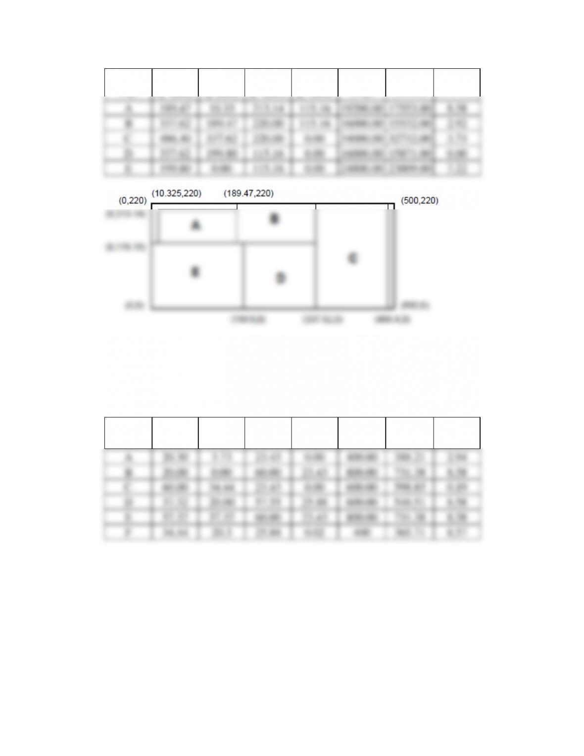
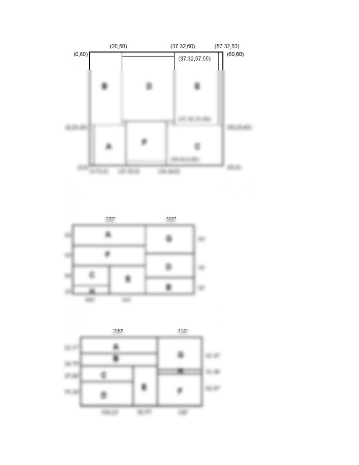
6.34 To avoid unrealistic department shapes, we set equal to two for all the departments. We
obtain the results shown in the following Table by using the linear MIP model given by
equations (6.21) through (6.37):
Dept xi“ (feet) xi‘ (feet) yi“ (feet) yi‘ (feet)
Area
(req.)
Area
(model)
Error (%)
A 189.47 10.33 213.14 115.16 19200.00 17553.00 8.58
B 337.62 189.47 220.00 115.16 16000.00 15532.00 2.92
C 486.40 337.62 220.00 0.00 34000.00 32732.00 3.73
D 337.62 199.80 115.16 0.00 16000.00 15871.00 0.00
E 199.80 0.00 115.16 0.00 24800.00 23009.00 7.22
Dept xi“ (feet) xi‘ (feet) yi“ (feet) yi‘ (feet)
Area
(req.)
Area
(model)
Error (%)
A 20.30 3.73 23.43 0.00 400.00 388.21 2.94
B 20.00 0.00 60.00 23.43 800.00 731.38 8.58
C 60.00 34.44 23.43 0.00 600.00 598.85 0.19
D 37.32 20.00 57.55 25.88 600.00 548.51 8.58
E 57.32 37.32 60.00 23.43 800.00 731.38 8.58
F 34.44 20.3 25.88 0.02 400 365.71 8.57
Answers to Problems at the End of Chapter 6 6-27
The objective value we obtained from the model is 2,130.70 units.
6.35 Using LOGIC to exchange departments B and F we obtain the following layout:
6.36 Using LOGIC to exchange departments D and H we obtain the following layout:
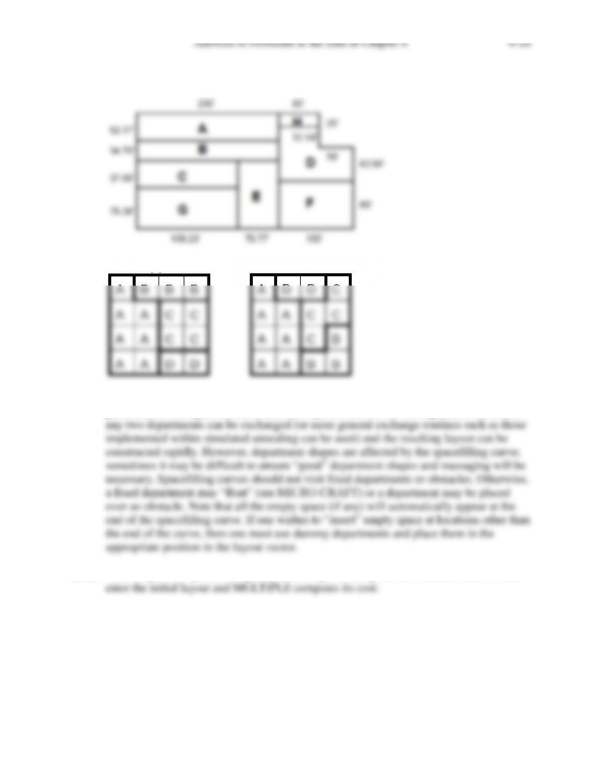
6.37 Using LOGIC to exchange departments G and H we obtain the following layout:
6.38a-b (a) (b)
6.38c A spacefilling curve “maps” or translates a two-dimensional problem (i.e., the layout
problem) into a single dimension (i.e., the layout vector or the fill sequence). Therefore,
6.39a Assuming a 1 x 1 grid for simplicity and using the data given for Problem 6.28, we first
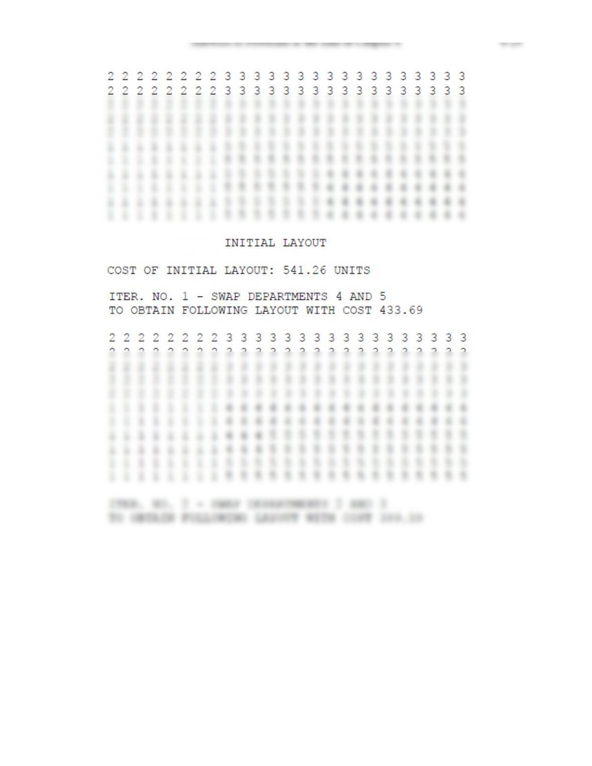
6.39b Using a conforming spacefilling curve may result in irregular department shapes,
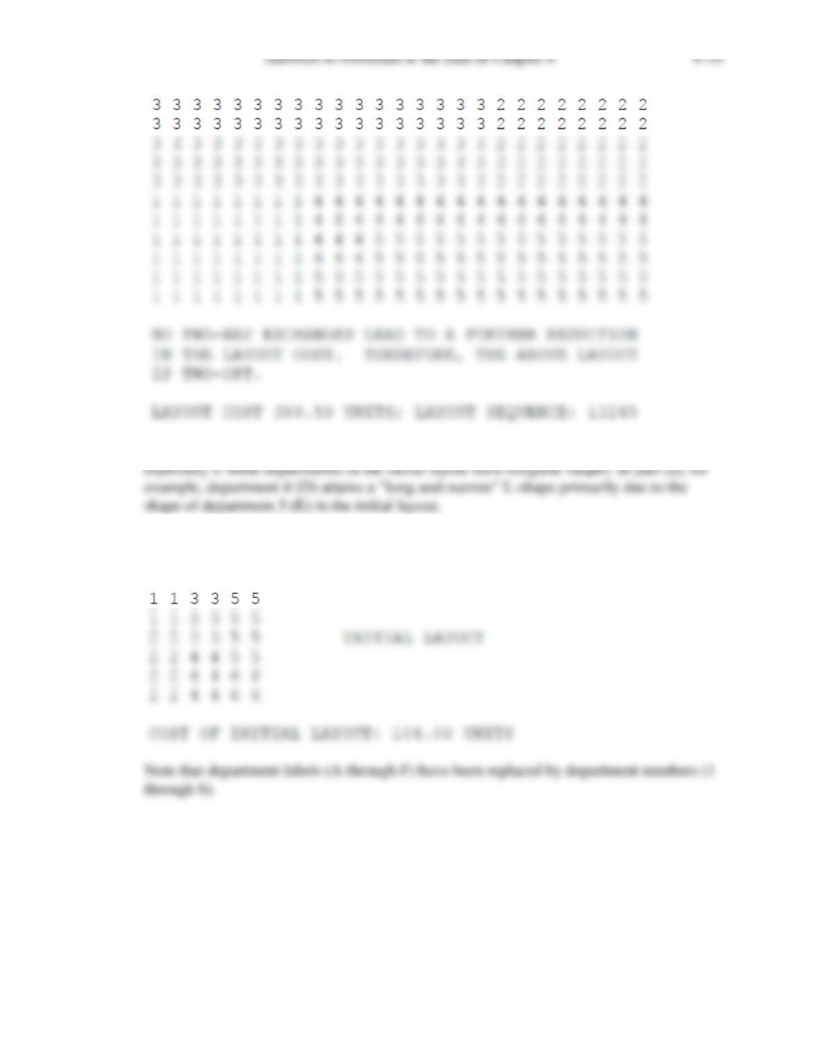
6.40 Assuming a 1 x 1 grid for simplicity and using the data given for Problem 6.29, we first
enter the initial layout and MULTIPLE computes its cost: