Answers to Problems at the End of Chapter 10 10-20
10.17 There was a mistake in the statement of the problem. It should have read, “Thirty percent
of the item movement between the existing machines and a new machine is between the
new machine and each of the existing machines at (0, 20) and (20, 0). Twenty percent is
between the new machine and each of the existing machines at (40, 0) and (0, 40).” The
following solution is based on the intended problem.
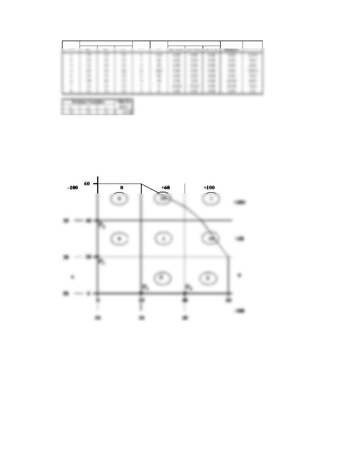
Existing machine locations are dock locations, the percentages represent the movement
between a dock and the storage location for an item, and the contour line is a continuous
representation of the storage boundary for the item. See Figure 7.19 for a discrete
representation of the storage boundary.
aibici|x – a i| |y – b i| |z – c i|
125 35 22 2 124 0.00 0.00 0.00 0.00 124.0
225 35 22 158 0.00 0.00 0.00 0.00 58.0
325 35 22 120 0.00 0.00 0.00 0.00 20.0
425 35 22 2 100 0.00 0.00 0.00 0.00 100.0
525 35 22 220 0.00 0.00 0.00 0.00 20.0
630 40 22 330 5.00 5.00 0.00 10.00 60.0
715 25 22 1 0 10.00 10.00 0.00 20.00 20.0
825 35 22 2 0 0.00 0.00 0.00 0.00 0.0
Obj Fn
x y z f(X*)
25 35 22 124.0
Rectilinear
Distance
gi+w idi
Decision Variables
Dept
coordinates
wi
gi
Absolute Difference
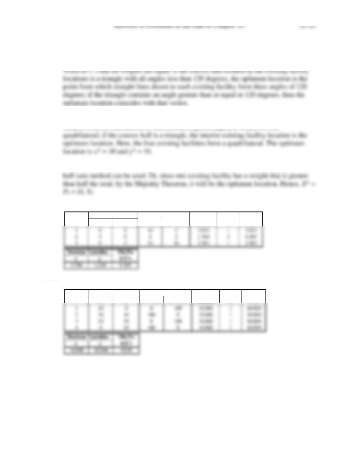
10.18a When one existing facility has at least half the total weight, its location is the optimum
location. This is knows as the Majority Theorem. Hence, X* = P2 = (5,0)
10.18b When all weights are equal and m = 4, if the convex hull is a quadrilateral, the optimum
location is at the intersection of lines connecting non-adjacent vertices of the
10.18c Since the convex hull is a straight line, the problem is a “location on a line” problem. The
10.19a
10.19b
EF Euclidean Weight
i
aibi(x – a i)2(y – b i)2Distance wiwidi
1 0 0 14 2 3.953 1 3.953
2 5 0 2 2 1.768 3 5.303
3 0 5 14 14 5.303 1 5.303
Obj Fn
x y
f(X*)
3.750 1.250 5.303
Coordinates
Squared Difference
Decision Variables
EF Euclidean Weight
i
aibi(x – a i)2(y – b i)2Distance wiwidi
110 0 0 100 10.000 1 10.000
220 10 100 0 10.000 1 10.000
310 20 0100 10.000 1 10.000
4 0 10 100 0 10.000 1 10.000
Obj Fn
x y
f(X*)
10.000 10.000 10.00
Decision Variables
Coordinates
Squared Difference
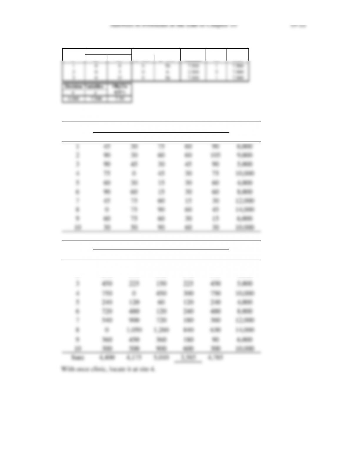
10.19c
10.20a
EF Euclidean Weight
i
aibi(x – a i)2(y – b i)2Distance wiwidi
1 0 0 0 56 7.500 1 7.500
2 0 5 0 6 2.500 3 7.500
3 0 15 056 7.500 1 7.500
Obj Fn
x y
f(X*)
0.000 7.500 7.50
Coordinates
Squared Difference
Decision Variables
Magisterial
District 1 2 3 4 5 Population
145 30 75 60 90 6,000
290 30 60 60 105 9,000
390 45 30 45 90 5,000
475 045 30 75 10,000
560 30 15 30 60 4,000
690 60 15 30 60 8,000
745 75 60 15 30 12,000
8 0 75 90 60 45 14,000
960 75 60 30 15 6,000
10 30 50 90 60 30 10,000
7540 900 720 180 360 12,000
8 0 1,050 1,260 840 630 14,000
9360 450 360 180 90 6,000
10 300 500 900 600 300 10,000
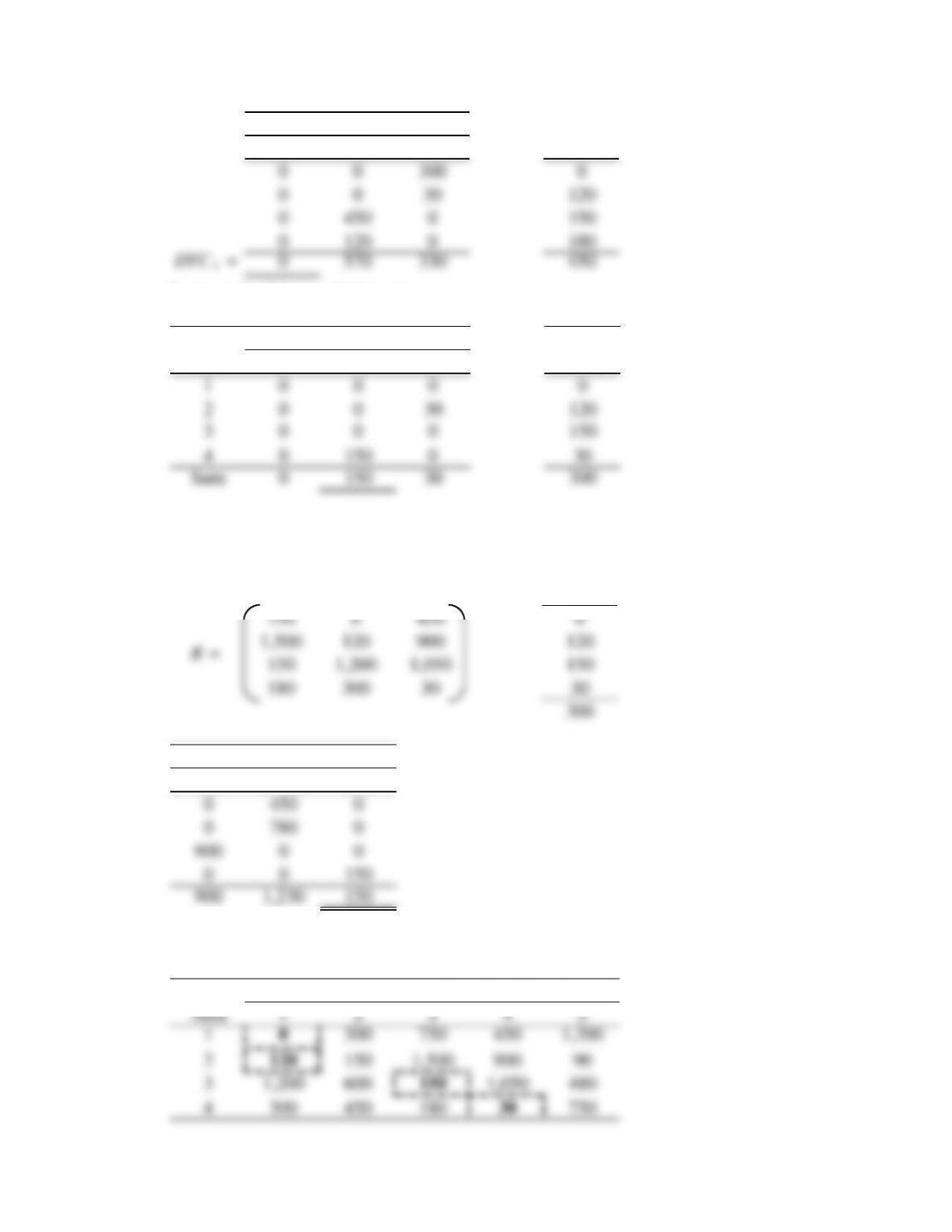
Sum: 4,400 4,175 5,010 3,585 4,785
Potential Sites
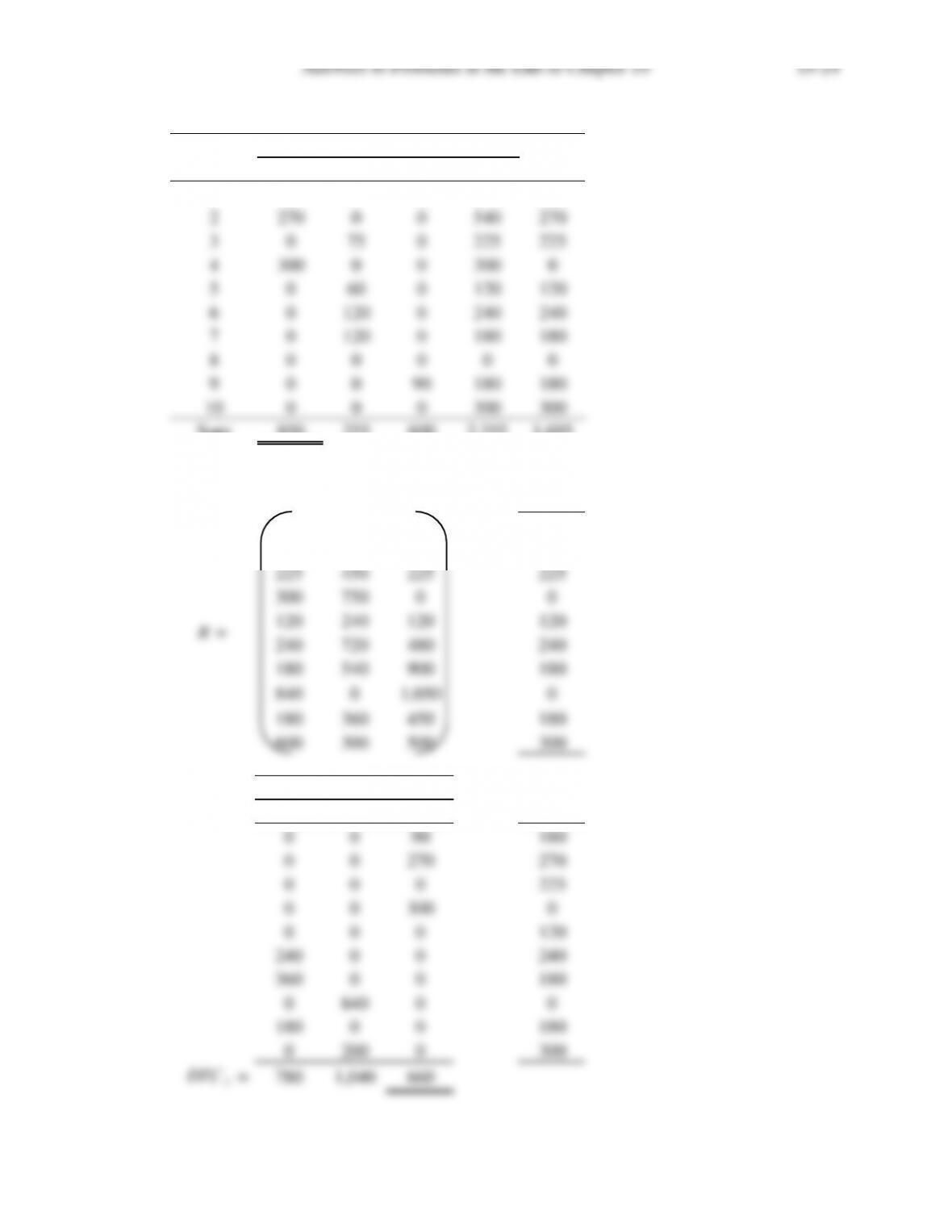
10.20b
With two clinics, locate them at sites 1 and 4.
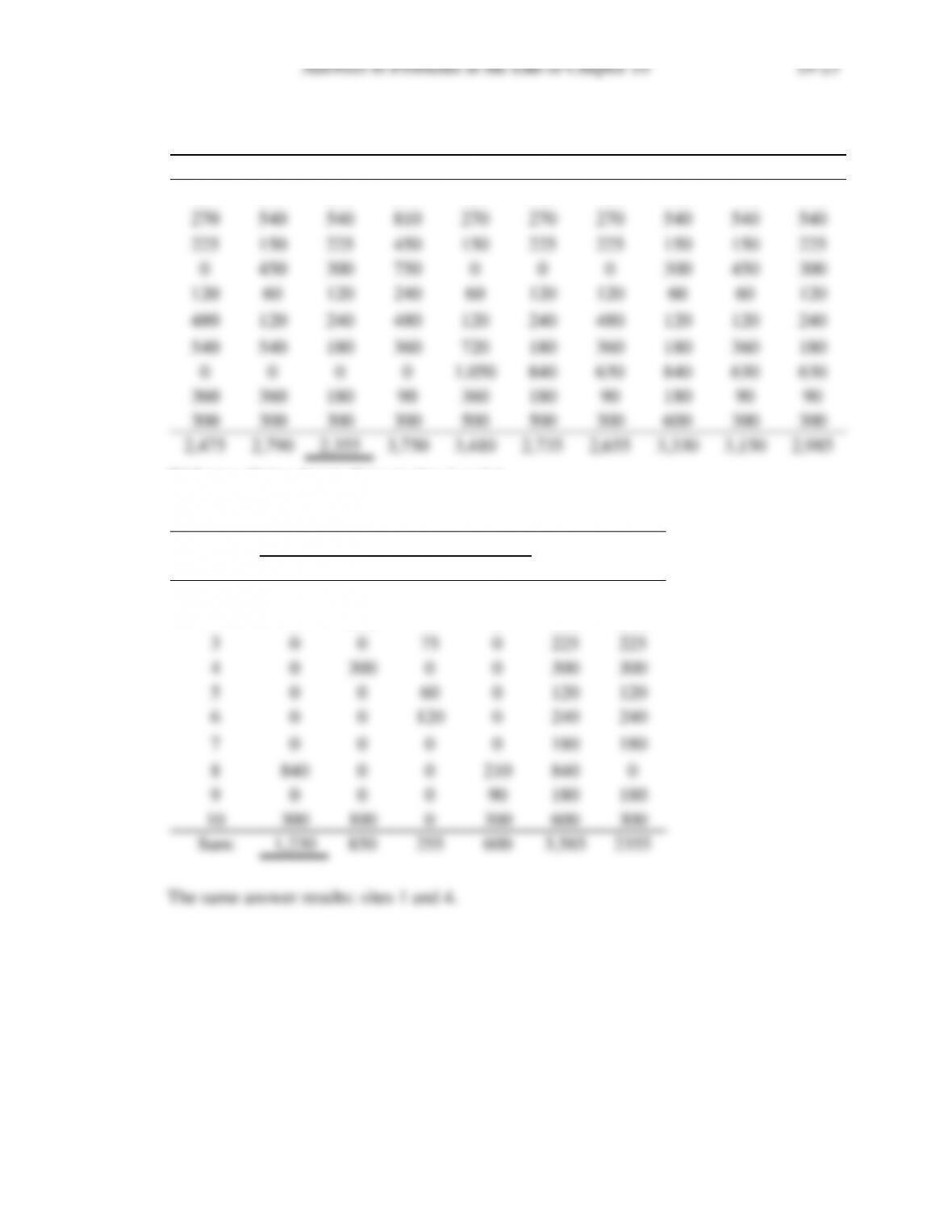
Using the Ignizio algorithm: theta x = 4:
1,2 1,3 1,4 1,5 2,3 2,4 2,5 3,4 3,5 4,5
180 270 270 270 180 180 180 360 450 360
270 540 540 810 270 270 270 540 540 540
225 150 225 450 150 225 225 150 150 225
0450 300 750 0 0 0 300 450 300
120 60 120 240 60 120 120 60 60 120
480 120 240 480 120 240 480 120 120 240
540 540 180 360 720 180 360 180 360 180
0 0 0 0 1,050 840 630 840 630 630
360 360 180 90 360 180 90 180 90 90
300 300 300 300 500 500 300 600 300 300
2,475 2,790 2,355 3,750 3,410 2,735 2,655 3,330 3,150 2,985
Magisterial
District 1 2 3 5 a* New a*
1 90 180 0 0 360 270
2 0 270 0 0 540 540
3 0 0 75 0 225 225
4 0 300 0 0 300 300
5 0 0 60 0 120 120
6 0 0 120 0 240 240
7 0 0 0 0 180 180
8 840 0 0 210 840 0
9 0 0 0 90 180 180
10 300 100 0 300 600 300
Sum: 1,230 850 255 600 3,585 2355
Potential Sites
10.20c
Magisterial
District 2 3 5 a* New a*
1 90 0 0 270 180
2 270 0 0 540 270
3 0 75 0 225 225
4 300 0 0 300 0
5 0 60 0 120 120
6 0 120 0 240 240
7 0 120 0 180 180
8 0 0 0 0 0
9 0 0 90 180 180
10 0 0 0 300 300
Sum: 850 255 600 2,355 1,695
Potential Sites
4 1 2
j1j2j3a*
360 270 180 180
540 810 270 270
225 450 225 225
300 750 0 0
120 240 120 120
240 720 480 240
180 540 900 180
840 0 1,050 0
180 360 450 180
600 300 500 300
R =
4 1 2 a*
0 0 90 180
0 0 270 270
0 0 0 225
0 0 300 0
0 0 0 120
240 0 0 240
ait
Answers to Problems at the End of Chapter 10 10-25
Since the once that is to be removed is the last one chosen, no removal is performed.
Also, since h = k, we stop.
10.21a
10.21b Same answer as for (a)
Magisterial
District 1 2 4
1 270 180 360
2 810 270 540
3 450 225 225
4 750 0300
5 240 120 120
6 720 480 240
7 540 900 180
801,050 840
9 360 450 180
10 300 500 600
Potential Sites
Magisterial
District 1 2 3 4 5
1 0 0 0 0 0
2 0 0 0 0 0
3 0 0 0 0 0
4 0 1 0 0 0
5 0 0 0 0 0
6 0 0 0 0 0
7 0 0 0 0 0
8 1 0 0 0 0
9 0 0 0 0 0
10 0 0 0 0 0
Potential Sites
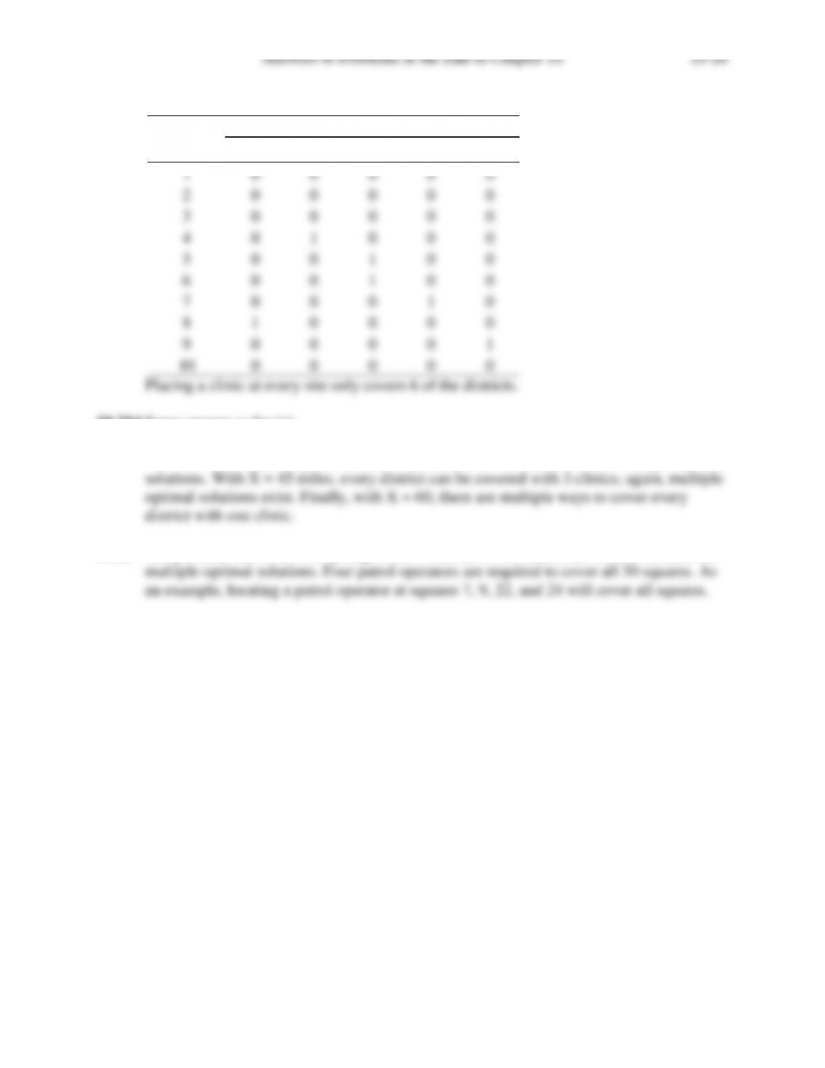
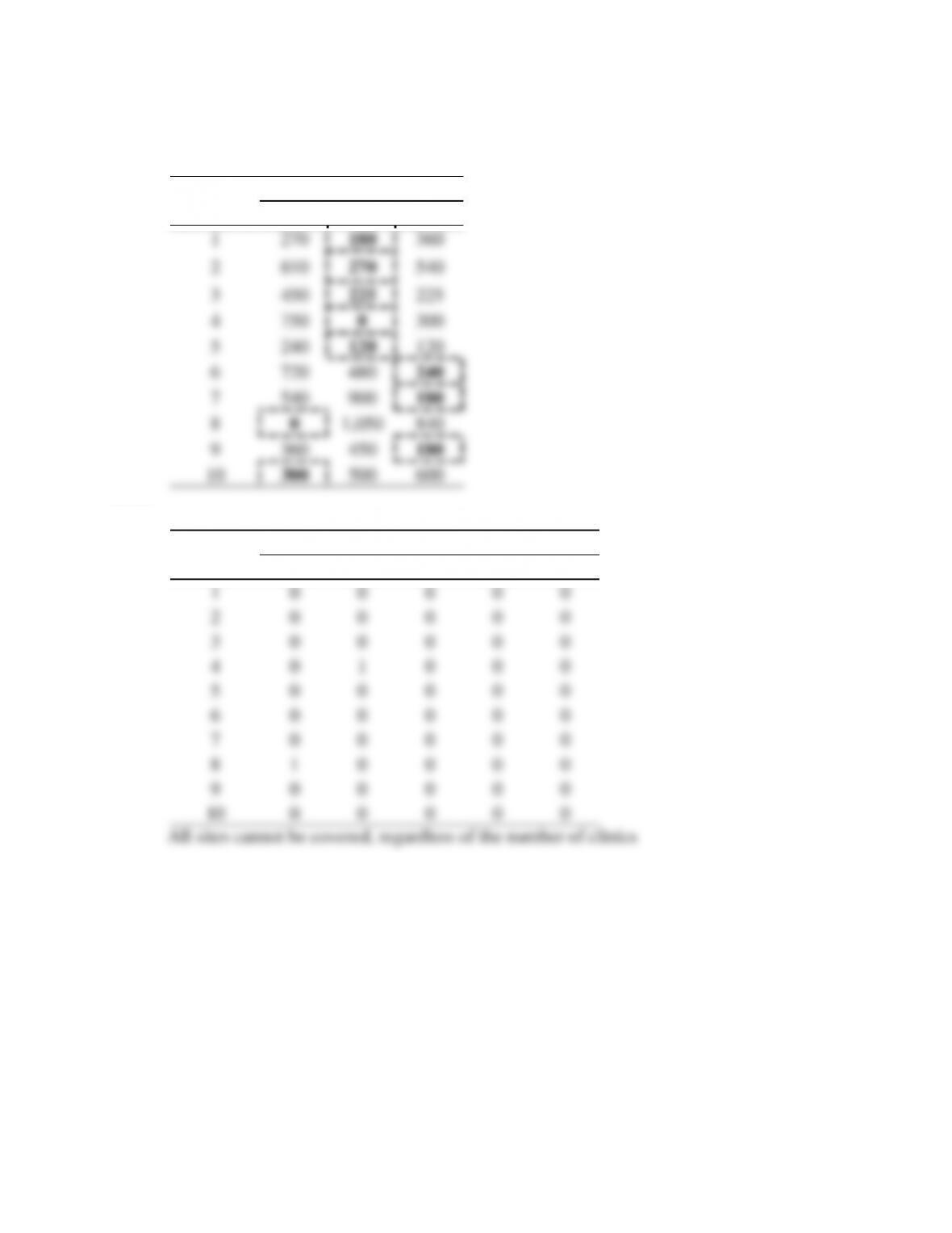
10.21c
10.21d Same answer as for (c)
With X = 30 miles, every district can be covered with 4 clinics; there are multiple optimal
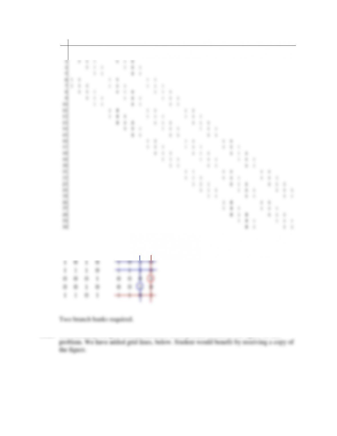
10.22 The problem can be solved by inspection. From the cover matrix shown below, there are
Magisterial
District 1 2 3 4 5
1 0 0 0 0 0
2 0 0 0 0 0
3 0 0 0 0 0
4 0 1 0 0 0
5 0 0 1 0 0
6 0 0 1 0 0
7 0 0 0 1 0
8 1 0 0 0 0
9 0 0 0 0 1
10 0 0 0 0 0
Potential Sites
Answers to Problems at the End of Chapter 10 10-27
10.23
1 2 3 4 5 6 78910 11 12 13 14 15 16 17 18 19 20 21 22 23 24 25 26 27 28 29 30
1 1 1 11
2 1 1 1 111
3 1 1 1 111
4 1 1 1 1 11
5 1 111
6 1 1 111 1
7 1 1 1 111 1 1 1
8 1 1 1 1111 1 1
9 1 1 1 1 11 1 1 1
10 1111 1 1
11 111 1 1 1
12 1111 1 1 1 1 1
13 1111 1 1 1 1 1
14 111 1 1 1 1 1 1
15 11 1 1 1 1
16 1 1 1 1 1 1
17 111 1 1 1 1 11
18 1 1 1 111 111
19 1 1 1 1 1 1 1 11
20 11 1 1 11
21 1 1 111 1
22 1 1 1 111 1 1 1
23 111 1111 1 1
24 1 1 1 1 11 1 1 1
25 1111 1 1
26 111 1
27 111111
28 1111 1 1
29 111 1 1 1
xx
1 0 1 0 1 0 1 0
Answers to Problems at the End of Chapter 10 10-28
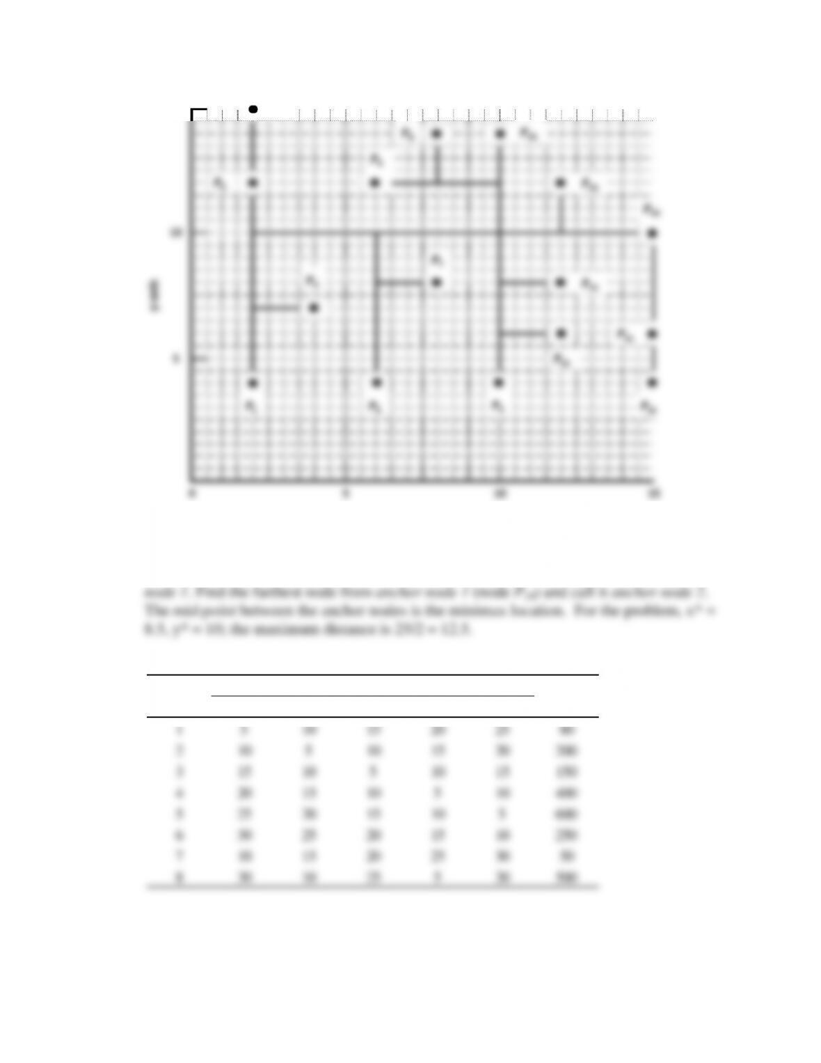
10.24a Using the majority algorithm, locate at x = 10 and y = 10.
10.24b Choose any node (say P8) and find the farthest node (which is node P1) and call it anchor
10.25a
10
15
5
10
0
5
x-axis
y-axis
15
P3
P2
P1
P5
P9
P14
P15
P11
P12
P16
P13
P10
P8
P6
P7
P4
# Trips
Customer 1 2 3 4 5 Weekly
1 5 10 15 20 25 80
210 510 15 20 200
315 10 510 15 150
420 15 10 510 400
525 20 15 10 5600
630 25 20 15 10 250
710 15 20 25 30 50
830 10 25 520 500
Potential Sites
Answers to Problems at the End of Chapter 10 10-29
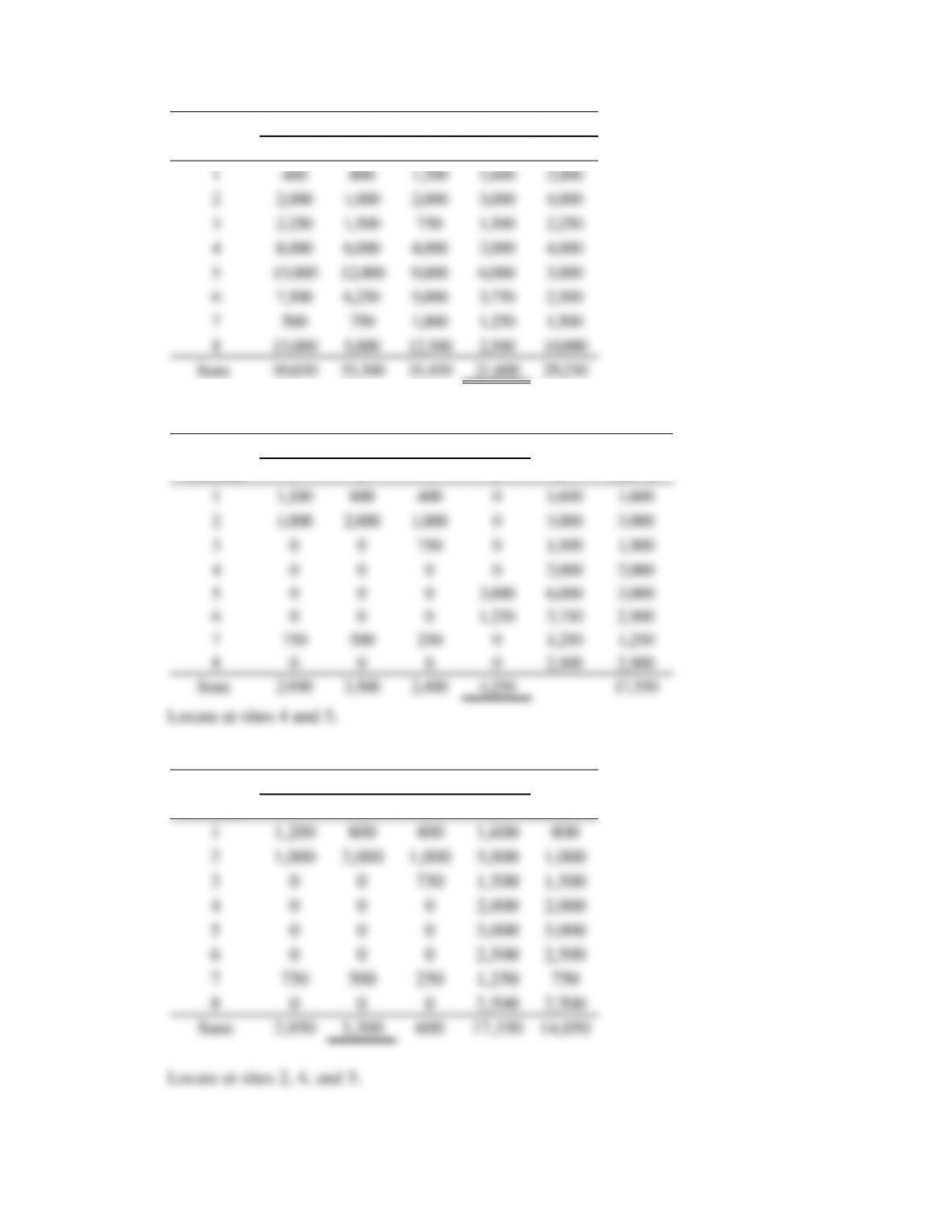
Locate at site 4.
10.25b
Customer 1 2 3 4 5
1400 800 1,200 1,600 2,000
2 2,000 1,000 2,000 3,000 4,000
3 2,250 1,500 750 1,500 2,250
4 8,000 6,000 4,000 2,000 4,000
5 15,000 12,000 9,000 6,000 3,000
6 7,500 6,250 5,000 3,750 2,500
7500 750 1,000 1,250 1,500
8 15,000 5,000 12,500 2,500 10,000
Sum: 50,650 33,300 35,450 21,600 29,250
Potential Sites
Customer 1 2 3 5 a* New a*
1 1,200 800 400 0 1,600 1,600
2 1,000 2,000 1,000 0 3,000 3,000
3 0 0 750 0 1,500 1,500
4 0 0 0 0 2,000 2,000
5 0 0 0 3,000 6,000 3,000
6 0 0 0 1,250 3,750 2,500
7750 500 250 0 1,250 1,250
8 0 0 0 0 2,500 2,500
Sum: 2,950 3,300 2,400 4,250 17,350
Potential Sites
Customer 1 2 3 a* New a*
1 1,200 800 400 1,600 800
2 1,000 2,000 1,000 3,000 1,000
3 0 0 750 1,500 1,500
4 0 0 0 2,000 2,000
5 0 0 0 3,000 3,000
6 0 0 0 2,500 2,500
7 750 500 250 1,250 750
8 0 0 0 2,500 2,500
Potential Sites
Answers to Problems at the End of Chapter 10 10-30
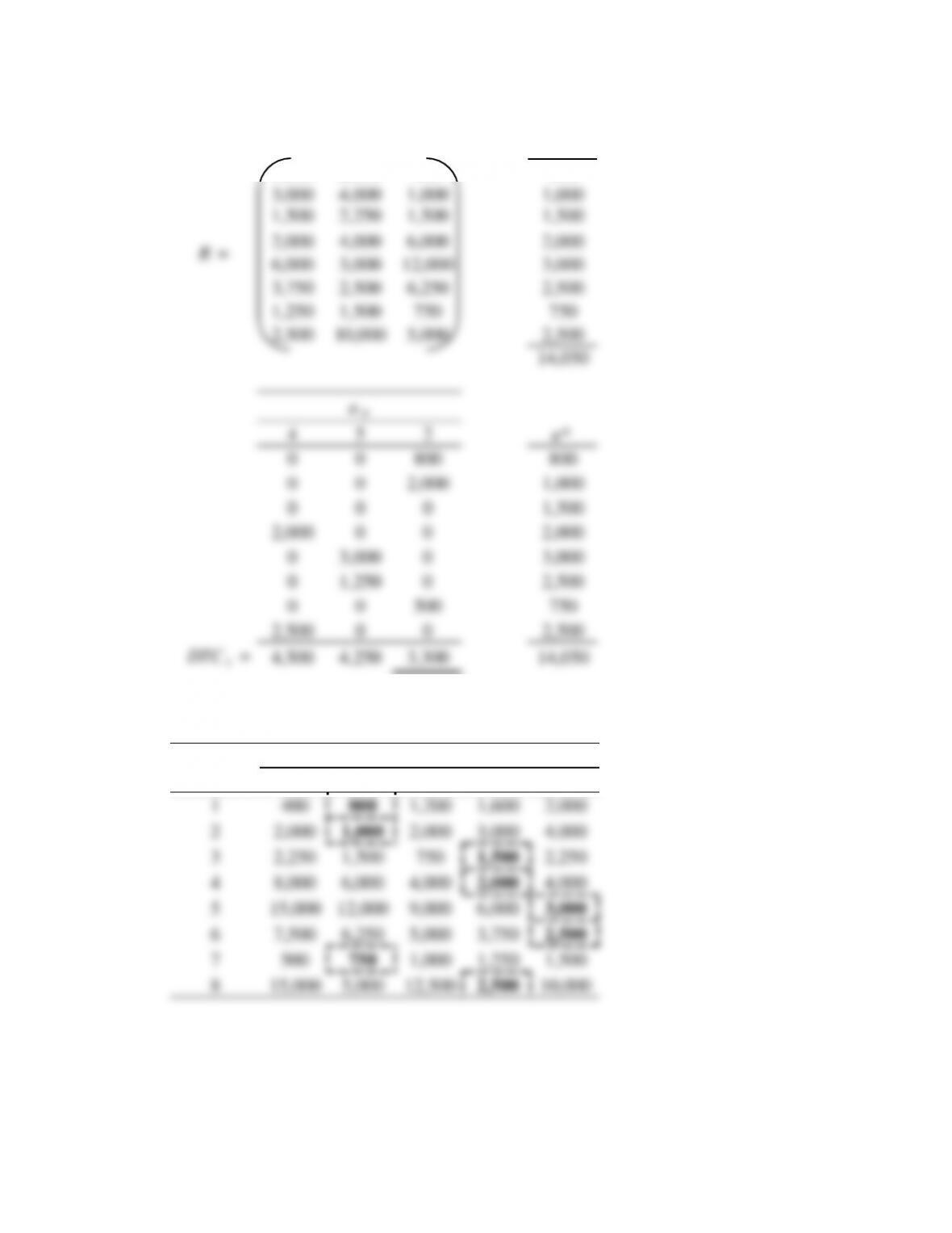
Since site 2 was just added to the set, we stop. Locate at 2, 4, and 5. Obj. fcn. = 14,050.
4 5 2
j1j2j3a*
1,600 2,000 800 800
3,000 4,000 1,000 1,000
1,500 2,250 1,500 1,500
2,000 4,000 6,000 2,000
6,000 3,000 12,000 3,000
3,750 2,500 6,250 2,500
1,250 1,500 750 750
2,500 10,000 5,000 2,500
14,050
R =
4 5 2 a*
0 0 800 800
0 0 2,000 1,000
0 0 0 1,500
2,000 0 0 2,000
0 3,000 0 3,000
0 1,250 0 2,500
0 0 500 750
2,500 0 0 2,500
DTC t = 4,500 4,250 3,300 14,050
ait
Customer 1 2 3 4 5
1 400 800 1,200 1,600 2,000
2 2,000 1,000 2,000 3,000 4,000
3 2,250 1,500 750 1,500 2,250
4 8,000 6,000 4,000 2,000 4,000
5 15,000 12,000 9,000 6,000 3,000
6 7,500 6,250 5,000 3,750 2,500
7 500 750 1,000 1,250 1,500
8 15,000 5,000 12,500 2,500 10,000
Potential Sites
10.26
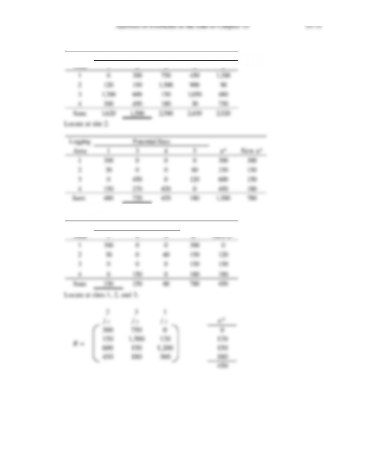
Locate at sites 2 and 3.
Logging
Area 1 2 3 4 5
1 0 300 750 450 1,200
2120 150 1,500 900 90
3 1,200 600 150 1,050 480
4300 450 180 30 750
Sum: 1,620 1,500 2,580 2,430 2,520
Potential Sites
Logging
Area 1 3 4 5 a* New a*
1300 0 0 0 300 300
230 0 0 60 150 150
3 0 450 0120 600 150
4150 270 420 0450 180
Sum: 480 720 420 180 1,500 780
Potential Sites
Logging
Area 1 4 5 a* New a*
1300 0 0 300 0
230 060 150 120
3 0 0 0 150 150
4 0 150 0180 180
Sum: 330 150 60 780 450
Potential Sites
Answers to Problems at the End of Chapter 10 10-32
Remove site 2 from solution set.
Locate at sites 1, 3, and 4.
Since site 4 was just added to the set, we stop. Locate at sites 1, 3, and 4.
Obj. fcn. = 300.
2 3 1 a*
0 0 300 0
0 0 30 120
0450 0150
0120 0180
DTC t = 0570 330 450
ait
Logging
Area 2 4 5 New a*
1 0 0 0 0
2 0 0 30 120
3 0 0 0 150
4 0 150 030
Sum: 0 150 30 300
Potential Sites
3 1 4
j1j2j3a*
750 0450 0
1,500 120 900 120
150 1,200 1,050 150
180 300 30 30
300
R =
3 1 4
0450 0
0780 0
900 0 0
0 0 150
900 1,230 150
ait
Logging
Area 1 2 3 4 5
10300 750 450 1,200
2120 150 1,500 900 90
31,200 600 150 1,050 480
4300 450 180 30 750
Potential Sites
10.27
Logging
Area 1 2 3 4 5
1 0 450 1,125 675 1,800
2180 225 2,250 1,350 135
31,800 900 225 1,575 720
4450 675 270 45 1,125
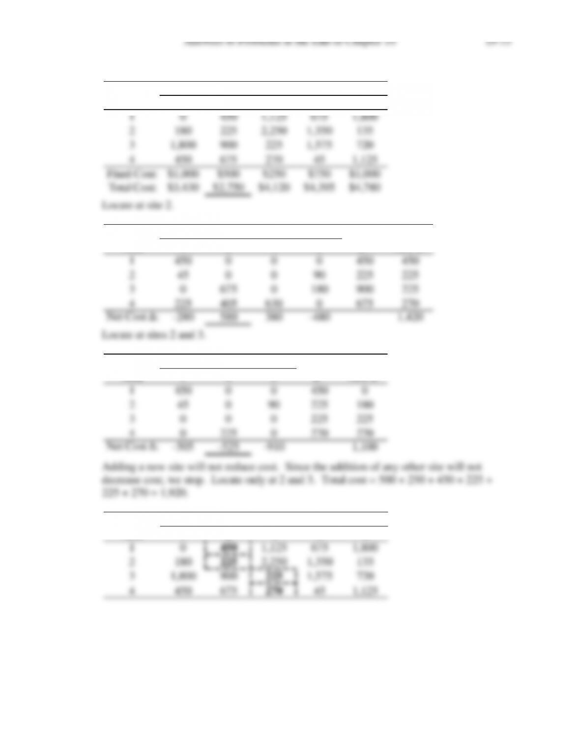
Fixed Cost: $1,000 $500 $250 $750 $1,000
Total Cost: $3,430 $2,750 $4,120 $4,395 $4,780
Potential Sites
Logging
Area 1 3 4 5 a* New a*
1450 0 0 0 450 450
245 0 0 90 225 225
3 0 675 0180 900 225
4225 405 630 0675 270
Net Cost ∆:–280 580 380 –480 1,420
Potential Sites
Logging
Area 1 4 5 a* New a*
1450 0 0 450 0
245 090 225 180
3 0 0 0 225 225
4 0 225 0270 270
Net Cost ∆:–505 –525 –910 1,100
Potential Sites
Logging
Area 1 2 3 4 5
1 0 450 1,125 675 1,800
2180 225 2,250 1,350 135
31,800 900 225 1,575 720
4450 675 270 45 1,125
Potential Sites
Answers to Problems at the End of Chapter 10 10-34
SECTION 10.3
10.28a Order the values in V and D in a decreasing and increasing order, respectively.
10.28b Suppose that department i is located at site i in the current layout design:
10.29a Assuming rectilinear distance
Decreasing order of flow rate: v = (250,200,150,150,150,100,50,30,20,10,10,0,0,0,0)
Distance Matrix:
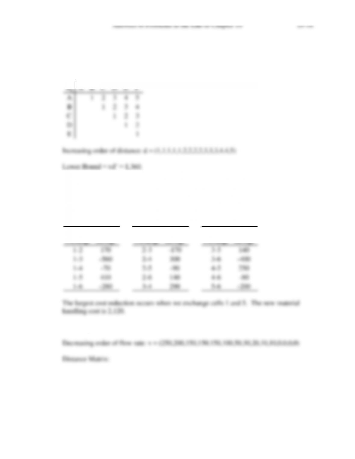
Increasing order of distance: d = (1,1,1,1,1,1,1,2,2,2,2,2,2,3,3)
10.29c There are 15 possible pairwise exchanges. For illustration purposes, only the first
iteration is shown.
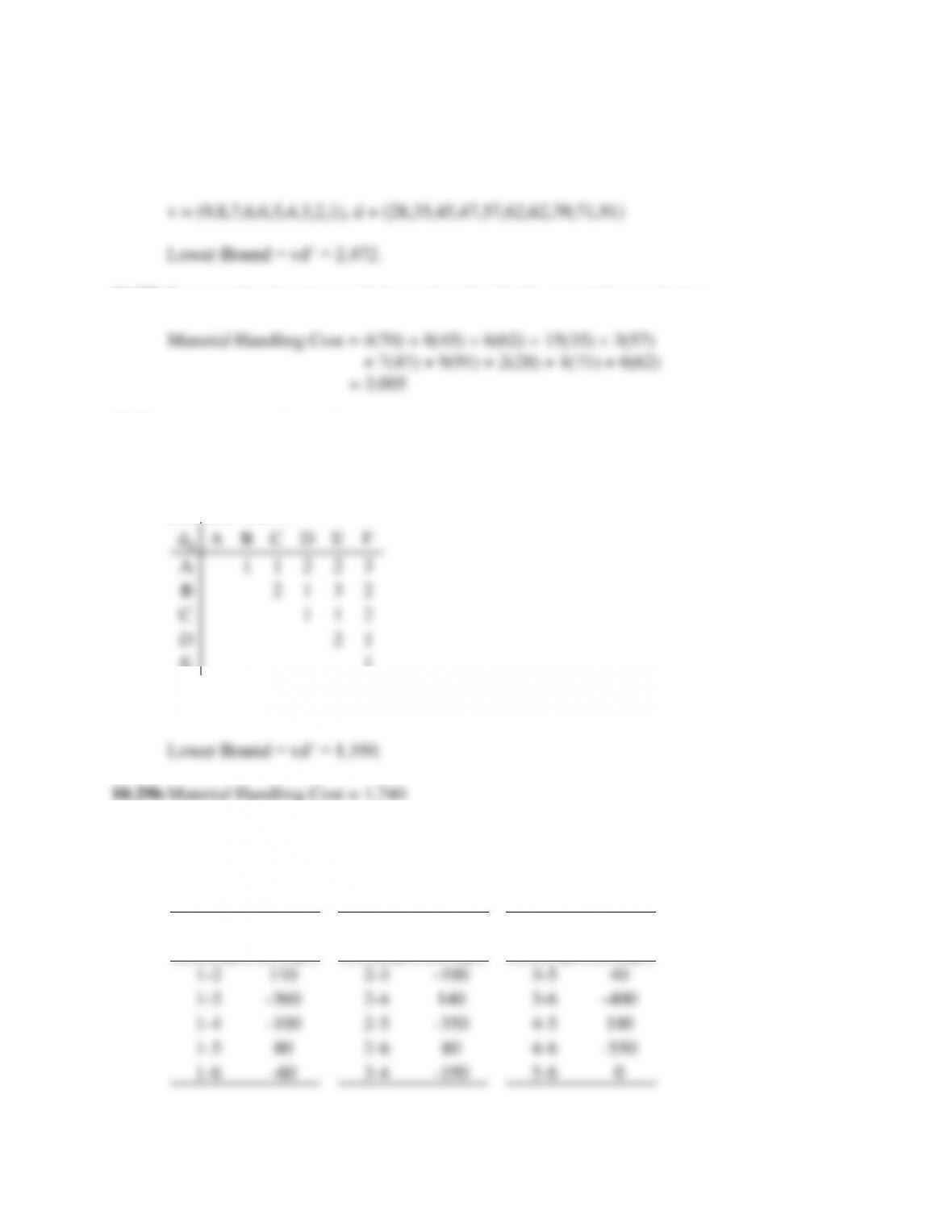
Iteration 1:
dij A B C D E F
A 1 1 2 2 3
B 2 1 3 2
C 1 1 2
D 2 1
E 1
Pairwise Pairwise Pairwise
Exchange Savings Exchange Savings Exchange Savings
1-2 110 2-3 –100 3-5 40
1-3 –360 2-4 140 3-6 –400
1-4 –100 2-5 –350 4-5 100
1-5 80 2-6 80 4-6 –550
1-6 –60 3-4 –190 5-6 0
Answers to Problems at the End of Chapter 10 10-35
The largest cost reduction occurs when we exchange cells 4 and 5. The new material
This problem illustrates the issues with choosing a starting point for the algorithm. The
algorithm will terminate in the second iteration without improving the solution obtained
from iteration 1. For instance, starting with the following initial arrangement will result
in a solution at the lower bound during the second iteration.
10.30a Assuming rectilinear distance
Decreasing order of flow rate: v = (250,200,150,150,150,100,50,30,20,10,10,0,0,0,0)
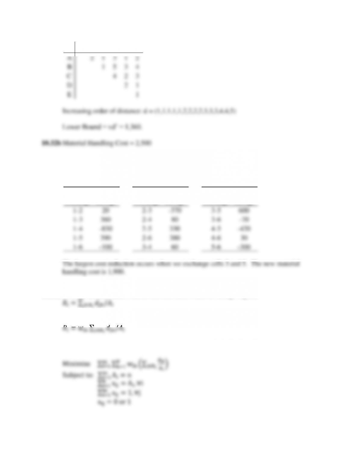
Distance Matrix:
Lower Bound = vd’ = 1,190.
10.30c There are 15 possible pairwise exchanges. For illustration purposes, only the first
iteration is shown.
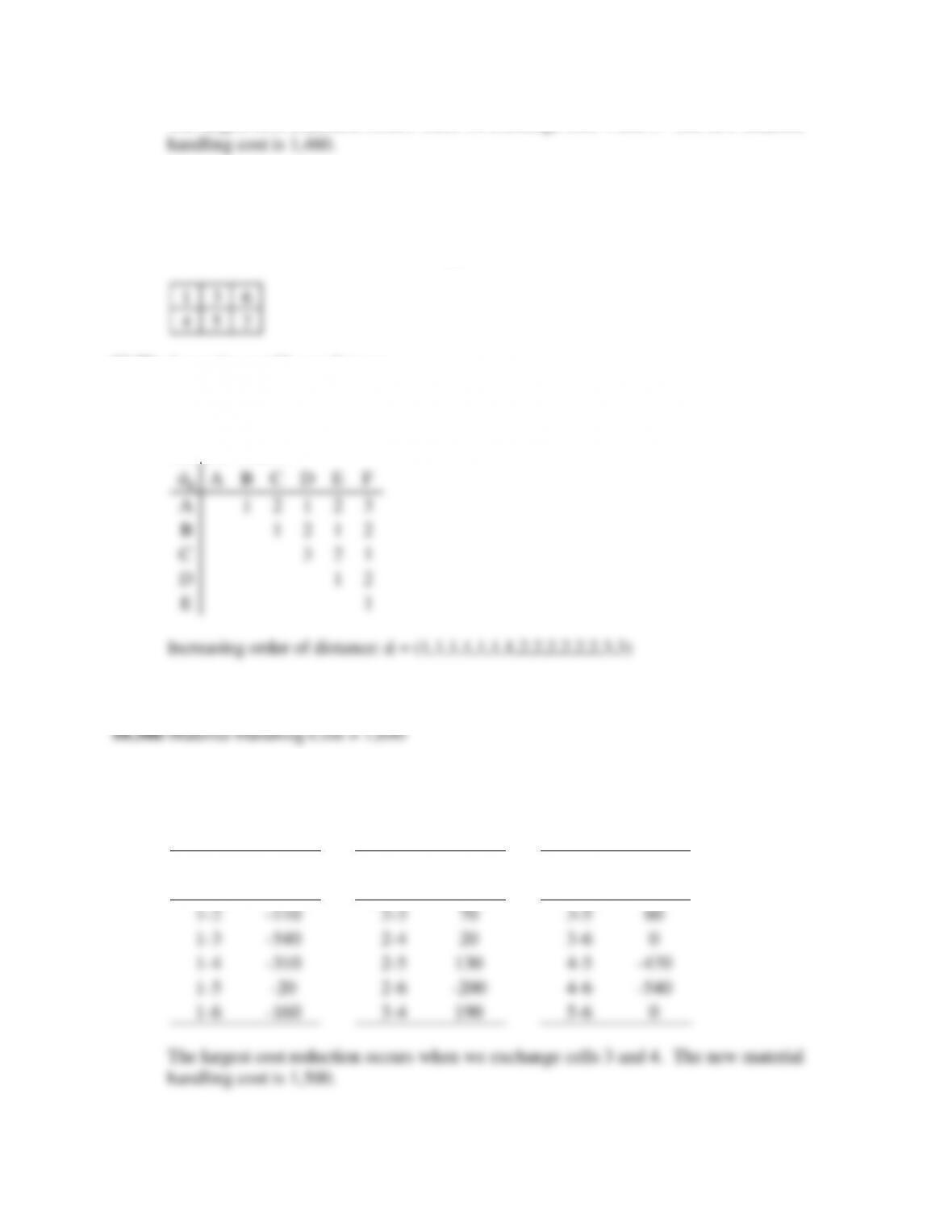
Iteration 1:
dij A B C D E F
A 1 2 1 2 3
B 1 2 1 2
C 3 2 1
D 1 2
E 1
Pairwise Pairwise Pairwise
Exchange Savings Exchange Savings Exchange Savings
1-2 –110 2-3 70 3-5 60
1-3 –540 2-4 20 3-6 0
1-4 –310 2-5 130 4-5 –470
1-5 –20 2-6 –200 4-6 –540
1-6 –160 3-4 190 5-6 0
10.31a Assuming rectilinear distance
Decreasing order of flow rate: v = (250,200,150,150,150,100,50,30,20,10,10,0,0,0,0)
Distance Matrix:
10.31b Material Handling Cost = 2,530
10.31c There are 15 possible pairwise exchanges. For illustration purposes, only the first
iteration is shown.
Iteration 1:
10.32a Assuming rectilinear distance
dij A B C D E F
A 1 2 3 4 5
B 1 2 3 4
C 1 2 3
D 1 2
E 1
Pairwise Pairwise Pairwise
Exchange Savings Exchange Savings Exchange Savings
1-2 170 2-3 –170 3-5 140
1-3 –560 2-4 300 3-6 –400
1-4 –70 2-5 –90 4-5 250
1-5 410 2-6 140 4-6 –80
1-6 –280 3-4 290 5-6 –200
Answers to Problems at the End of Chapter 10 10-37
10.32c There are 15 possible pairwise exchanges. For illustration purposes, only the first
iteration is shown.
Iteration 1:
10.33a Average distance item i travels between dock k and its storage region,
10.33b Average cost of transporting item i between dock k and its storage region,
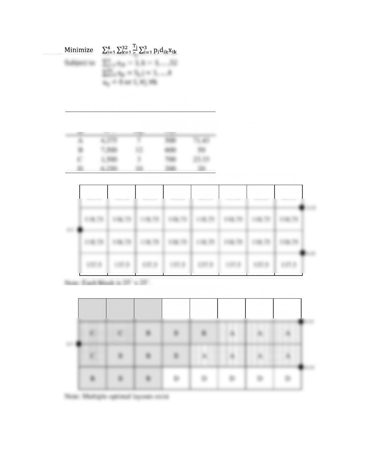
10.33c Integer programming formulation:
dij A B C D E F
A 2 1 3 1 2
B 1 5 3 4
C 4 2 3
D 2 1
E 1
Pairwise Pairwise Pairwise
Exchange Savings Exchange Savings Exchange Savings
1-2 20 2-3 –370 3-5 600
1-3 360 2-4 80 3-6 –70
1-4 –830 2-5 330 4-5 –420
1-5 390 2-6 380 4-6 30
1-6 –100 3-4 60 5-6 –300
Answers to Problems at the End of Chapter 10 10-38
10.34a
10.34b Product Ranking: C > A > B > D.
Product Area # of Bays Load Rate
Tj/Sj
(j)
(ft2)(Sj)(Tj)
A4,375 7500 71.43
B7,500 12 600 50
C1,500 3700 23.33
D6,250 10 200 20
137.5 137.5 137.5 137.5 137.5 137.5 137.5 137.5
118.75 118.75 118.75 118.75 118.75 118.75 118.75 118.75
118.75 118.75 118.75 118.75 118.75 118.75 118.75 118.75
137.5 137.5 137.5 137.5 137.5 137.5 137.5 137.5
0.5
0.25
0.25
B B B D D D D D
C C B B B A A A
C B B B A A A A
B B B D D D D D
0.5
0.25
0.25
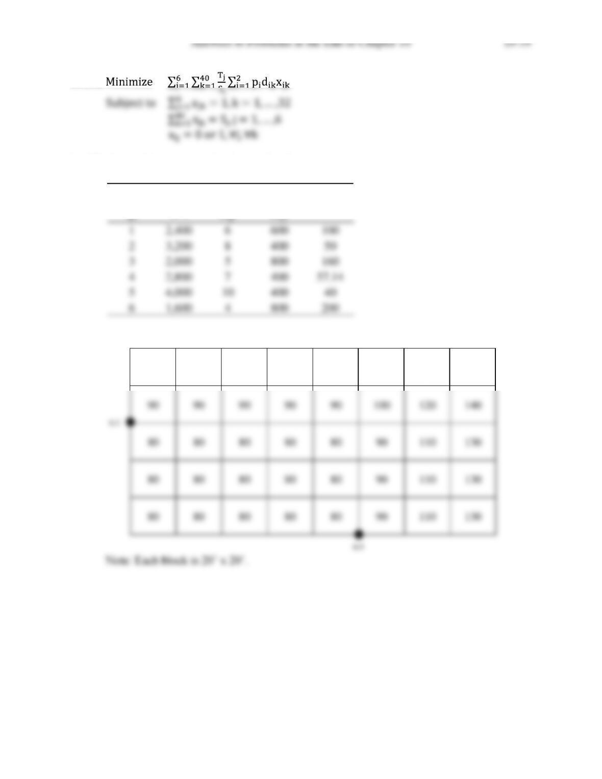
10.35a
10.35b Product Ranking: 6 > 3 > 1 > 4 > 2 > 5
Product Area # of Bays Load Rate
Tj/Sj
(j)
(ft2)(Sj)(Tj)
12,400 6600 100
23,200 8400 50
32,000 5800 160
42,800 7400 57.14
54,000 10 400 40
61,600 4800 200
110 110 110 110 110 120 140 160
90 90 90 90 90 100 120 140
80 80 80 80 80 90 110 130
80 80 80 80 80 90 110 130
80 80 80 80 80 90 110 130
0.5
0.5