CHAPTER 7
Simultaneous-Move Games: Mixed Strategies
Teaching Suggestions
This chapter introduces mixed strategies and the methods used to solve for mixed-strategy
equilibria in zero-sum and non-zero-sum games. For zero-sum games, students are likely to accept the
idea of randomization more readily if they think of it themselves. One way to lead them to the idea is to
present games in which a Nash equilibrium in pure strategies does not exist; in such games, it is important
for each player to conceal his choice from the other. Take the Tennis-Point game in Chapter 4 (Figure
4.14), and ask one student to put herself in the shoes of Evert and think whether she would choose
cross-court or down the line. Usually the answer will be one or the other, with some technical
justification. Then ask another student how she would react if she were Navratilova. Proceeding this way,
get them to realize the importance of keeping the other guessing. Similarly, to get across the idea of an
equilibrium in mixed strategies, a good way to start is by getting students to trace out the succession of
best responses that goes full circle in the tennis table or equivalent. The same can be done with any other
example you used previously, perhaps a soccer penalty kick. The advantage of these two is that you can
supplement your discussion by bringing in the evidence on successful mixing in these situations at the top
professional levels (Section 7.8 in the text). You can also remind your students how sports commentators
always speak of “mixing it up,” “keeping the defense honest,” or similar phrases for the general idea of
not acting in a pattern that the other side can detect and exploit.
If you showed the poison scene from The Princess Bride in your first class, you can remind the
students of that situation and carry out a similar discussion asking two students to take on the roles of
Westley and Vizzini. If you did not show the excerpt before, this is a good time to do so.
If you have plenty of time, and good computer and audiovisual facilities, you can take two
students and have them play such a game repeatedly, showing the choices and payoffs of each play
immediately on the projection screen. The class can then make suggestions to the players. This discussion
can evolve or be guided into the realization of the importance of mixing. Unlike in many other situations,
having the same two players play repeatedly in this zero-sum game facilitates each player’s detection of
any pattern of behavior the other might adopt and of ways to exploit that pattern to one’s own advantage
and the other’s detriment.
Once you have provided some intuition or motivation for the use (and usefulness) of mixed
strategies, you can approach the problem of solving for the equilibrium mixtures. Students will quickly
grasp the idea that mixed strategies are a special case of continuous strategies in which players choose a
value for p, the probability of using one of the two possible actions, from the interval [0, 1]. Most will
also see immediately that a value of p at 0 or 1 coincides with the use of a pure strategy.
We have been most successful motivating mixed-strategy equilibria by building on the intuition
developed above. That is, a good mixed strategy will guarantee that a player’s rival cannot choose one
pure strategy and use it to his advantage. You can explain this to your students in two ways. The first is
that the “right” mix, or the equilibrium value of p or q, ensures that one’s rival does not have a specific
pure strategy that is his (unique) best response to the mix. The second, equivalent, interpretation is that
the right mix guarantees that a player’s opponent gets the same payoff against the mix from all of his
available pure strategies; the opponent is indifferent among his available pure strategies. Using this
approach has the advantage that it can be easily extended to non-zero-sum games; it also follows
smoothly from a discussion of the value of mixing.
The method of best responses, or “opponent’s indifference,” is developed in Section 2 of the
chapter. You can use your example of a game with no pure strategy equilibrium and add a row and
column to the table for the p– and q-mixes. In the table, the row for the p-mix and the column for the
q-mix contain payoffs for all possible values of p or q against the rival’s pure strategies. These payoffs are
represented as functions of p or q and, as such, can be graphed. Once you graph, say, the column player’s
payoffs as a function of the row player’s choice of p, students will be able to see (literally) that for most
values of p, the column player has a pure strategy as his best response to row’s mixture. Only when the

payoff lines from column’s two pure strategies cross does his best response include both pure strategies
and any weighted average of the two, that is, any mix over those pure strategies. Most students are easily
convinced by the visual information provided in the graph and can better understand the concept of an
equilibrium mix as a result.
1. Example of a Zero-Sum Game
When it comes to the actual formal analysis, one example that we have used successfully in class
for the basic two-by-two zero-sum mixing case is based on the Sherlock Holmes–Moriarty story that is
told in von Neumann and Morgenstern’s Theory of Games and Economic Behavior (Princeton, N.J.:
Princeton University Press, 1944), pp. 176–178. The gist of the story is that Holmes is trying to get from
London via Canterbury to Dover by train (and hence to the continent) in order to escape from Moriarty.
Moriarty has seen Holmes enter the train and can presumably get another himself. Each must then decide
whether to go all the way to Dover or to get out at the single intermediate station at Canterbury; Holmes
would prefer to make the opposite decision from Moriarty, while Moriarty would prefer to make the same
decision as Holmes.
Many students will not have read the story. For that matter, many may not be entirely familiar
with the geography of England and France. [One of us (Dixit) has used a schematic drawing of the
southeast corner of England showing the cities in question, the Channel, and the northern coast of France
to make a joke about the modern student’s ignorance of geography.] It may be worthwhile to add a bit of
background related to Conan Doyle and the Holmes stories as well as Moriarty, who was not only the
“godfather” of crime in London but a professor of mathematics as well.
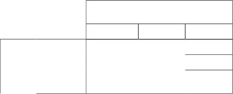
The payoff table we have used for this game follows:
Holmes
Dover Canterbury
Moriarty
Dover 75 0
Canterbury –50 100
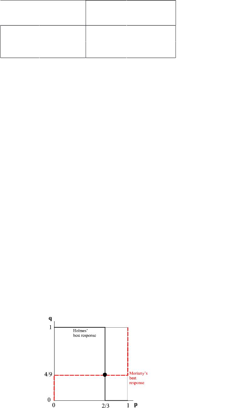
Graphing payoffs for Moriarty playing his pure strategies against Holmes’s q-mix allows you to derive
Moriarty’s best response to different values of q that Holmes could choose. (Earlier editions of the text
include graphs of this type. For an example, see Figure 7.2 from the third edition. Values of Holmes’s q
are measured on the horizontal axis with Moriarty’s payoff on the vertical axis. Each of Moriarty’s pure
strategies generates a line on the graph.) For small values of q, the line associated with Moriarty’s choice
of Canterbury (intercept 100 at q = 0 and –50 at q = 1) is higher, indicating that the pure-strategy
Canterbury is his best response. For large values of q, Moriarty’s choice of Dover (intercept 0 at q = 0 and
75 at q = 1) is his best response. Moriarty is indifferent among his pure strategies only when the lines
intersect; the value of q at the intersection solves 75q = –50q + 100(1 – q) to give an optimal q of 4/9.
Moriarty’s expected payoff when q = 4/9 is –331/3 (and Holmes’s payoff is 331/3). A similar analysis can
be conducted to find Holmes’s best responses to various values of p chosen by Moriarty. The
best-response curves for the two players in this game show only one equilibrium for the game and that is
the equilibrium in mixed strategies for p = 2/3 and q = 4/9. These best-response curves are illustrated
below:
You can extend this example to one in which Holmes has three pure strategies (although this goes
beyond the scope of the analysis in von Neumann and Morgenstern). Here Holmes has a third strategy,
Emergency, which is to pull the train’s emergency stop cord somewhere between Canterbury and Dover
and to exit the train in this way. This strategy also forces Moriarty’s trailing train to stop when it discovers
the track ahead blocked. What are the payoffs from this new strategy? If Moriarty has gotten off at
Canterbury, then for Holmes, Emergency is obviously better than Canterbury but worse than Dover
because it still leaves him in the interior and not immediately on the boat to France; hence Emergency
gets Holmes 0 if Moriarty gets off at Canterbury. But if Moriarty goes on to Dover, then his train will be
held up due to the train emergency, and Holmes will find Emergency better than Dover but worse than
Canterbury; we give Holmes a –20 (and Moriarty a 20) for this combination. Then we get the following
payoff matrix, with a row added for Moriarty’s p-mix:
Holmes
Dover Canterbury Emergency
Moriarty
Dover 75 0 20
Canterbury –50 100 0
p-mix:
pD + (1 – p)C
75p – 50(1 – p) 100(1 – p) 20p
Moriarty’s minimum payoffs here no longer create an inverted V shape as p varies from 0 to 1
because Holmes has three strategies. Rather, we see Moriarty’s set of minimum payoffs as the thick line
in the diagram below:
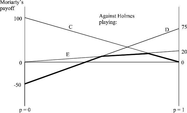
The
maximin value of
p chosen by
Moriarty is the one
that yields the
highest point on
the thick line in the
diagram, or the p at the intersection of Holmes’s C(anterbury) and E(mergency) lines. That p solves 20p =
100(1 – p); p = 5/6. Moriarty’s maximin payoff is 100/6 = 16 2/3.
Note that Moriarty’s mix would be better against Holmes’s use of the pure-strategy Dover but
Holmes does not use Dover in his mix. Holmes chooses C and E with probabilities z and (1 – z). The
equilibrium value of z solves 0z + 20(1 – z) = 100z + 0(1 – z), which yields z = 20/120 = 1/6. Holmes’s
minimax payoff is 100/6 = 50/3, which is the same as Moriarty’s maximin.
2. Example of a Non-Zero-Sum Game
Getting students to accept and understand the idea of mixing in non-zero-sum games is even
harder than in zero-sum games. In zero-sum games, if one player fails to mix correctly, the other can
exploit this mistake to her own advantage, entailing an immediate loss to the first player. That is usually
not the case in non-zero-sum games. Indeed, many senior game theorists do not accept (or at least dislike)
mixed strategies in this context. If you share that view, you may choose to omit this material entirely.
Here are some suggestions on how to proceed if you want to cover this material.
We are now fortunate to have one non-zero-sum game that engages the students’ interest to the
extent that they are likely to want to pursue its analysis all the way to finding a mixed-strategy
equilibrium. This is the “beautiful blonde” game from the bar scene in the movie A Beautiful Mind. In
Chapter 4 of this manual we presented its analysis. Mathematically, it is a game of chicken, and therefore
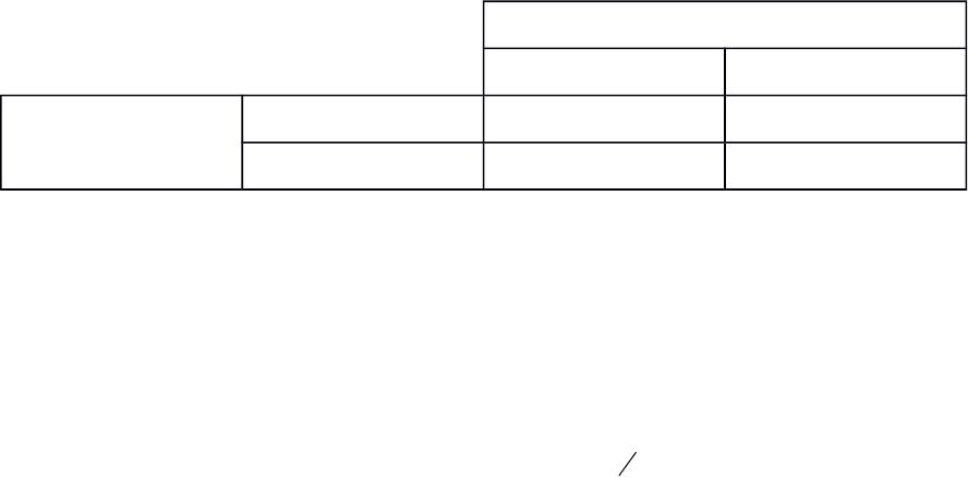
has an equilibrium in mixed strategies. The payoff matrix presented in Chapter 4 is reproduced below:
Male 2
Blonde Brunette
Male 1
Blonde 1, 1 4, 2
Brunette 2, 4 3, 3
Using this table, it is easy to see that Player 1’s p-mix (probability p of choosing Blonde and [1 – p] of
choosing Brunette) keeps Player 2 indifferent if
12
1 (1 ) 4 2 (1 ) 3
(1 )(4 3) (2 1)
1 .
p p p p
p p
p p
´ + – ´ = ´ + – ´
– – = –
– = =
You can ask students for suggestions as to how the payoff numbers could be different from the ones given
in our matrix, and calculate how the mix changes in response.
You can even generalize this game to one in which n males choose between one blonde and n (or
more) brunettes. Then the game is mathematically similar to the game of Helping Someone in Need
(Chapter 11, Section 5). Suppose that for each player the payoff is 4 from winning the blonde (this
happens if he is the only one choosing Blonde), 3 from winning a brunette when none of the others wins
the blonde, 2 from winning a brunette when one of the other men wins the blonde, and 1 from losing out
altogether (when two or more males choose the blonde). Consider a symmetric, mixed-strategy
equilibrium, where p is the probability that any one male chooses Blonde, and the choices are independent
across players. Then any one player must be indifferent given the mixes of all the others. This requires
4(1 – p)n–1 + 1[1 – (1 – p)n–1] = 2(n – 1)p(1 – p)n–2 + 3[1 – (n – 1)p(1 – p)n–2].

Note that the payoff of 2 is multiplied by the probability that exactly one of the other (n – 1) players
chooses Blonde and (n – 2) choose Brunette. Rearranging terms, this indifference condition becomes
(1 – p)n–2 [ 3 + np – 4p] = 2.
The left-hand side is a decreasing function of p. When p = 0, it equals 3; when p = 1, it equals 0.
Therefore, there is a unique p between 0 and 1 that solves the equation. When n = 2, we have 3 – 2p = 2,
or p = ½, verifying the previous calculation. For other n, we need a numerical solution.
We can also ask: What is the probability that no one chooses the blonde? When each of n people
independently randomizes, choosing one of the brunettes with probability (1 – p), the probability that all
the men go for brunettes is (1 – p)n. Call this q.
Here is a table of solutions for p and q corresponding to various values of n:
n1 2 3 4 5 6 10 20
p1 0.500 0.268 0.183 0.139 0.113 0.064 0.030
q0 0.250 0.392 0.446 0.473 0.487 0.516 0.543
Perhaps surprisingly, the more suitors there are, the higher the probability that the blonde is totally
ignored by them all! The reason is that the probability that any one of them chooses her goes down very
fast as their numbers increase, and this outweighs the fact that there are more of them. A similar example
is developed in Chapter 11, Section 5.
For added interest, you can ask students to do similar solutions, and calculate the effects of
changing the underlying payoffs, using some other scale instead of the ranking 1 to 4. Most science
students carry sophisticated calculators these days and can solve such problems very fast.
A variant of this beautiful blonde game is presented in Exercise S14 at the end of the chapter. For
that exercise, we have simplified the payoff structure for the game, using the same payoffs as those in
Exercise S13 in Chapter 4. (The major difference is that the payoff to “no girl” is 0 in the exercises.)
Students with a certain level of math background may find the mathematics in the exercise easier than
that required to do the example as we have described it here.
If you can bring a laptop equipped with Gambit to your classroom, you can solve even more
complex games on the spot. For example, you can take the Soccer Penalty Kick game of Section 7, ask
the students for suggestions on how the strategies or the payoffs might differ from the numbers in the text,
and display the resulting equilibrium immediately. If you can hook up the computer so that the monitor
screen can be directly shown on the class screen, the effect is more dramatic.
If your class is sufficiently sophisticated in mathematics, then you can develop some of the ideas
and techniques presented in the online appendices to this chapter. Here are a few suggestions: