978-0393919684 Chapter 16 Lecture Note

Unlock access to all the studying documents.

View Full Document

CHAPTER 16

Bidding Strategy and Auction Design

Teaching Suggestions

Most students nowadays will have used some Internet auction sites, certainly as

buyers, and several as sellers. You can start a discussion related to their own experiences and

bring in the appropriate terminology as appropriate. In this way, you should be able to address

the differences between common-value and private-value auctions and between sealed bid and

open outcry; students may also be familiar with first and second price, as well as ascending and

descending auction mechanisms. And you will be able to elicit many of the strategies, fair and

fraudulent, that are used to manipulate the outcomes of auctions.

For the winner’s curse, you can play the auction as a penny-jar game, described below,

or think of a different example in which the low bid wins. House painters and other service

providers often participate in such low-bid auctions. A painter will come up with her estimate

of the time necessary to do the job, add in the cost of the predicted necessary materials, and

submit a bid. In these situations, the painter (and the purchaser of the service) can verify the

quantity of materials used, so she can ask that these costs be covered in full even if they

exceed (by some limited amount) the amount stated in the original bid. But the painter cannot

ask her client to cover the costs of additional time under most such bids, because of the moral

hazard problems involved. Suppose the true time needed to sand and paint a house is 14

person-days of time (assuming every painter has the same abilities). Then each painter makes

an estimate of the time it will take her, and each estimate will come with some error (within 2

or 3 days on either side of 14, for example). If lots of painters make bids and these are all

pooled, their arithmetic average would be an unbiased and probably pretty accurate indicator of

the true time needed to do the job. But each painter has only her own estimate, and the lowest

of these will be biased on the short side (2 or 3 days short of 14). Thus, if a homeowner

chooses the lowest bid, the winning painter is likely to have bid too little and will find that she

has to use more time than anticipated in completing the job. Here the painter wins a job only

when her rivals make estimates higher than hers. You could ask your students about ways to

combat this problem. For instance, what if all house painters looked ahead to the winner’s

curse and adjusted their bids upward to compensate for the bias?

The revenue equivalence outcome is another example that can be used successfully in

class. The text notes that expected outcomes under all four primary types of auctions are

identical when bidders are risk neutral and their valuations are independent, but goes on to note

that more-advanced mathematical techniques are needed to prove this result.

In an English auction, the person who places the higher value on the item, call this

value VA, will win it. Given that VA is the higher valuation, the other bidder’s valuation VB is

equally likely to be anywhere between 0 and VA. On average, therefore, the lower valuation VB

= VA/2. Since the lower bidder drops out of the auction at VB = VA/2, the bidder with the higher

valuation wins the item, pays (on average) VA/2, and receives an expected profit equal to VA –

VA/2 = VA/2.

Now, suppose the same people are bidding on the item using a first-price sealed-bid

auction. Obviously, the bidders will shade their bids below their true values. The question is By

how much? Since the bidders are risk neutral, each will act in a way that maximizes expected

profit = (person’s probability of winning)(person’s value – person’s bid). Without deriving the

optimal bids from scratch, it can be shown that a Nash equilibrium bidding outcome entails

each bidder’s submitting a bid equal to half his valuation.

To show that this strategy is a Nash equilibrium, assume that Bidder 2 uses it, and

therefore submits a bid equal to B2 = V2/2. We must then demonstrate that Bidder 1’s optimal

response is to adopt the same strategy. To show this, note that Bidder 1’s probability of

winning the auction equals Prob(B1 > B2). Given Bidder 2’s assumed strategy, this probability

equals Prob(B1 > V2/2), which can be rewritten as Prob(V2 < 2B1). Since we’ve assumed that

valuations are equally likely to be anywhere between 0 and 1, the probability that V2 < 2B1

(assuming that B1 is less than or equal to 1/2) equals 2B1. Thus (given Bidder 2’s assumed

strategy), the probability that Bidder 1’s bid of B1 will be the higher bid (and will thus win the

auction) equals 2B1. If Bidder 1 does submit the higher bid, her profit from doing so will be (V1

– B1). We can therefore say that Bidder 1’s expected profit = (probability of winning)(value –

bid) = 2B1(V1 – B1) = 2(B1V1 – B12). The remaining step is for Bidder 1 to choose B1 in a way that

maximizes her expected winnings. (One could employ a calculus-based approach, using a

simple derivative, to show that Bidder 1’s expected winnings are maximized when V1 – 2B1 = 0,

or B1 = V1/2. Such an approach has a critical flaw, however, because the bidder’s payoff

function is not accurate at any outcome that would entail a bid over 0.5. The formula is based

on the probability of winning the auction equaling 2V1; obviously, this formula is in error for B1

> 0.5, although it turns out that there is never any reason for Bidder 1 to bid more than 0.5. The

optimality of the B = V/2 strategy is not altered by this complication, but a correct derivation of

the optimal bidding strategy is more complicated than the simple derivative would suggest.)

To avoid the difficulties inherent in applying calculus to the problem, a series of tables

of possible bids can be used to show that the optimal bid is B1 = V1/2. The procedure is to

assume that Bidder 2 uses the bidding strategy B2 = V2/2, assume a particular value for V1, and

determine Bidder 1’s optimal bid. Suppose, for example, that B2 = V2/2, V1 = 0.4, and Bidder 1

bids 0.1. Bidder 1 will win the auction with probability 0.2 (since B1 = 0.1 > B2 only if V2 < 0.2)

and will collect earnings of 0.4 – 0.1 = 0.3 if she does. Her expected earnings using this bid are

thus (0.2)(0.3) = 0.6. The following table shows how Bidder 1 would do if she used some other

possible bids:

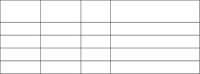
Bid

Probability

of win

Profit

Expected profit =

(probability of win)(profit)

0.10 0.2 0.20 0.060

0.15 0.3 0.25 0.075

0.20 0.4 0.20 0.080

0.25 0.5 0.15 0.075

0.30 0.6 0.10 0.060

Under these assumptions, it is clear that B1 = 0.2 is the best bid; note that this bid follows the

rule B1 = V1/2.

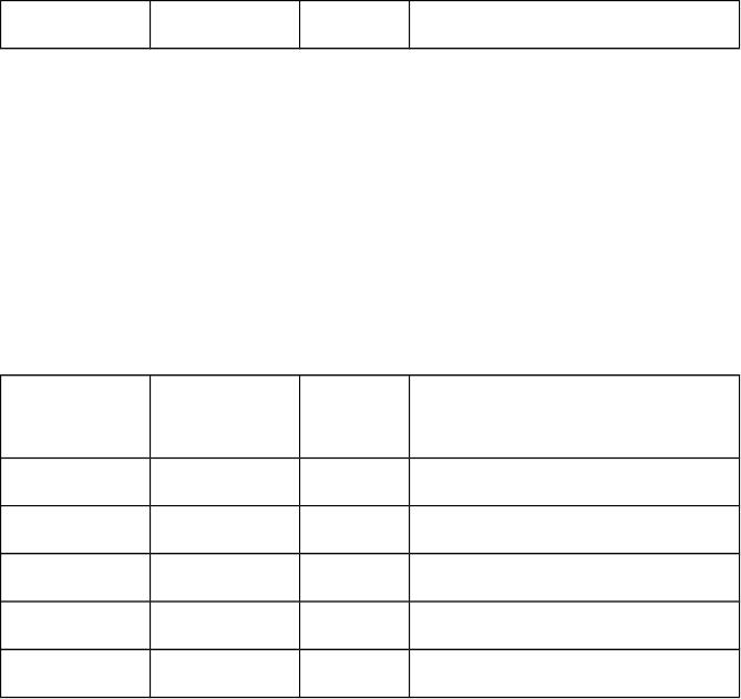
Now, consider other possible values for V1; for example, V1 = 0.6. In this case (again

assuming that B2 = V2/2), a table like the above reads:

Bid

Probability

of win

Profit

Expected profit =

(probability of win)(profit)

0.20 0.4 0.40 0.160

0.25 0.5 0.35 0.175

0.30 0.6 0.30 0.180

0.35 0.7 0.25 0.175

0.40 0.8 0.20 0.160

Again, the optimal bid follows the rule B1 = V1/2.

One last example, assuming that V1 = 0.9:

Bid

Probability

of win

Profit

Expected profit =

(probability of win)(profit)

0.35 0.7 0.55 0.385

0.40 0.8 0.50 0.400

0.45 0.9 0.45 0.405

0.50 1.0 0.40 0.400

Again, the optimal bid is B1 = V1/2. (Note that the above table only has four entries because

[given Bidder 2’s assumed strategy] there is never any reason for Bidder 1 to bid more than 0.5;

that bid guarantees that her bid will be the higher.)

In all of these examples, we see that Bidder 1’s optimal strategy is to bid B1 = V1/2. The

same conclusion holds for other possible values of V1. We can thus conclude that an outcome in

which each person bids an amount equal to half of her evaluation is a Nash equilibrium; when

B2 = V2/2, Bidder 1 wants to set B1 = V1/2 (and Bidder 2’s incentive is the same).

Finally, consider a bidder’s expected winnings in this Nash equilibrium. Since both

bidders are following the same strategy, the bidder who places the highest valuation on the

good will win it. Furthermore, since the winning bid is equal to half the person’s valuation, the

person with the higher valuation will always collect winnings equal to exactly half his

valuation.

Remember our conclusion from the English auction case analyzed above. The bidder

(A) with the higher valuation (VA) wins the item, pays (on average) VA/2, and receives an

expected amount of profit equal to VA – VA/2 = VA/2. In the simple case we have analyzed,

therefore, we can see that (in equilibrium) the English auction and the first-price sealed-bid

auction produce identical outcomes in terms of expected value. The person who values the

object the most always wins it and pays, either on average (in the English auction) or with

certainty (in the first-price sealed-bid auction), a price equal to half of her valuation of the

object.

We already know that with risk-neutral bidders and independent valuations (in

equilibrium), the first-price, sealed-bid auction produces an outcome identical to that of the

Dutch auction, while the English auction produces an outcome identical to that of a sealed-bid

second-price auction. The conclusion that the first-price sealed-bid auction and the English

auction produce identical outcomes (in this case) thus establishes the equivalence of all four

auction designs.

If you want to go more deeply into the Internet auction case study, you may want to

distribute funds to your students to use to purchase an actual item on eBay or some other

online auction site. Many, many items can be purchased for surprisingly small amounts

(although shipping fees can add considerably to the final price). Another possibility is to

discuss the bidding program used at eBay. The instructions at the site describe the bidding

program (“proxy bidding”) as a way to simulate an English auction (although eBay doesn’t use

that term) between interested bidders. The eBay procedure can (not surprisingly) also be

viewed as a way to conduct a second-price sealed-bid auction with an increment added to the

second-highest bid. Students could be asked to write (for hypothetical posting on the eBay site)

a new description that explains the eBay bidding procedure in terms of a second-price

sealed-bid auction. For listings and information about other auction sites on the Internet, see

http://online-auction-sites.toptenreviews.com or www.internetauctionlist.com.

For those who want to consider other auction-related issues, another possibility is to

pursue in greater detail the Clark-Groves public goods valuation revelation scheme to

supplement or buttress the discussion of Vickrey and second-price auctions. This connection is

mentioned briefly in the text, but the details of the Clark-Groves scheme are found in many

intermediate microeconomics texts; for example, see H. Varian, Intermediate Microeconomics,

9th ed. (New York: W. W. Norton, 2014), pp. 730–735. We also provide a number of different

in-class games that can be used to address a variety of topics from Vickrey’s truth serum to the

derivation of the optimal bid in an all-pay auction.

Game Playing in Class

GAME 1—Auctioning a Penny Jar (Winner’s Curse)

This game was discussed as a possible game for the first or second day of class (see

Chapters 1 and 2). Show a jar of pennies; pass it around so each student can have a closer look

and form an estimate of the contents. Show the students a stack of 100 pennies to give them a

better idea of what the jar might contain. While the jar is going around, explain the rules.

Everyone plays and each submits a sealed bid; hand out blank cards and ask students to write

down their names and bids and return the cards. The winner will pay his bid and get money

(paper and silver, not pennies) equal to that in the jar. Ties for a positive top bid split both prize

and payment equally. When you explain the rules, emphasize that the winner must pay his bid

on the spot in cash.

After you have collected and sorted the cards, write the whole distribution of bids on

the board. Our experience is that if the jar contains approximately $5.00, the bids average to

$3.50 (including a few zeros). Thus the estimates are on the average conservative. But the

winner usually bids about $6.00. Hold a brief discussion with the goal of getting across the idea

of the winner’s curse.

GAME 2—All-Pay Auction of $10

This game was also discussed as a possible game for the first or second day of class.

Everyone plays. Show students a $10 bill, and announce that it is the prize; the known value of

the prize guarantees that there is no winner’s curse. Hand out cards. Ask each student to write

down his name and a bid (in whole quarters). Collect the cards. The highest posi tive bid wins

$10; if two or more tie with the highest positive bids, they share the $10 equally. All players

pay the instructor what they bid, win or lose.

Be sure to emphasize before bids are submitted that “This is for real money; you must

pay your bid in cash on the spot. You can make sure of not losing money by writing $0.00. But

of course if almost everyone does that, then someone can win with $0.25 and walk away with a

tidy profit of $9.75.”

Once you have collected the cards, write the distribution of bids on the board. Hold a

brief discussion about the distribution and the value of the optimal bid. This game usually leads

to gross overbidding; a profit of $50 in a class or section of 20 is not uncommon. If that

happens, you will have to find ways of returning the profit to the class; we have done this by

having a party if the sum is large enough or by bringing cookies for the next meeting if the sum

is small. Of course, do not announce this plan in advance.

You can follow this game with a relatively in-depth discussion of the optimal bid in an

all-pay auction. If your students are comfortable with the necessary mathematics, you could go

on to derive the formula for the optimal bid.

GAME 3—Common-Value Asset Auction

Tell your students to imagine that you own an asset. The value to you of this asset is

some number between 0 and 100 points. All values from 0 to 100 are equally likely to be the

asset’s value.

Whatever this asset is worth to the instructor, it is worth 1.5 times that amount to each

student. Thus, the value to the student of this asset is some number between 0 and 150 points

(each possible value is equally likely). Students are asked to make a bid for this asset. The

instructor will sell the asset to a student if and only if the student’s bid is larger than the asset’s

value to the instructor.

Students can receive points (or cash) from this game in two ways: the first outcome

will involve luck, the second will be the average outcome. For the first outcome, the instructor

will use a random-number table to choose a number between 0 and 100, which will be the

value to her of the asset. Anybody who bids more than that value buys the asset and pays the

number of points (or pennies) he bid; anybody who bids less than the amount found in the table

does not buy the asset. If a student buys the asset, the gain or loss of points (or pennies) is

computed as the asset’s value to the student minus the amount paid to buy it. (Instructors can

use the same asset value to compute each student’s gain or loss of points [or pennies]. A

student’s gain or loss depends on the amount bid and on the randomly selected value of the

asset.) For the second outcome, students will receive the expected value of their bids, which is

the average number of points per game that they would be expected to have if this game were

repeated a number of times.

The results from this game can be used to lead a discussion about issues related to

common-value auctions. (There are also ways in which this game can be construed as a type of

coordination game if students are concerned not only about the outcome from their own bid but

about how all other students fare in acquiring points from the game.)

GAME 4—Puppy Auction

The following is based on an auction experiment used by Bob Weber in a course on

strategic decision making at Northwestern University. Tell students:

Suppose that you are one of two collectors involved in the sealed-bid

auction of a classic 1997 “Spot” Beanie Baby puppy. This Spot is worth $V to

you (you will determine V precisely below). Thus, you would be indifferent

between losing Spot to your rival bidder and paying $V for Spot.

Having sized up your opponent, you think Spot could be worth

anything between $0 and $100 to her. (She has probably sized you up

similarly.) The two valuations of the bidders in this auction are subjective—

primarily matters of taste—and therefore we will assume that they are

independent. This means that the value you assign to Spot will not affect your

assessment of your rival’s valuation. (For instance, if you have a valuation of

$95, this does not change your opinion about your rival’s being equally likely

to value Spot at any value from $0 to $100.)

The seller (the instructor) will unseal both bids, and will sell Spot to

the high bidder. We will consider two different pricing rules: (1) under the first

set of rules, the seller will collect from the winner a price (in points or pennies)

equal to that bidder’s bid; and (2) under the second set of rules, the seller will

collect from the winner a price (in points or pennies) equal to the lower, losing

bid.

To make it worthwhile to win the auction, all winning bidders will

receive 10 points for each dollar of profit made on their purchase. Profit is

defined as the difference between your V and the price you pay if you win the

auction. In addition, you will all calculate a pair of values and will make two

bids in each auction; this is to avoid discriminating against those with high

valuations.

You will be asked to use a piece of personal information to determine

the actual value of Spot to you. You will then be asked to consider several

questions pertaining to each type of auction.

HANDOUT FOR THIS GAME

Name: _____________________________________

Student ID number: __________________________

Your value 1 is found by taking the last two digits of your ID number.

Value 1: _______

Your value 2 is found by subtracting value 1 from 99.

Value 2: _______

First Auction

This is a standard sealed-bid auction, where the higher of the two submitted bids wins, and the

winner pays the amount she bid. Assume the value of Spot to you is value 1.

What will you bid for Spot? _________

How likely do you think it is that your bid will win? _______

(There are no points associated with the second question here.)

Now assume the value of Spot to you is value 2.

What will you bid for Spot? _________

How likely do you think it is that your bid will win? _______

Second Auction

This is an auction in which the higher of the two submitted bids wins, but the winner only pays

the amount of the (lower) losing bid.

Assume the value of Spot to you is value 1.

What will you bid for Spot? _________

How likely do you think it is that your bid will win? _______

Now assume that the value of Spot to you is value 2.

What will you bid for Spot? _________

How likely do you think it is that your bid will win? _______

Discussion of the results from these auction questions can be used to compare bidding

results in different auction types. Students can also consider the amount of shading that occurs

in different auctions and how bids may vary depending on the valuations of the bidders.