52 Chapter Highlights
Chapter 22
Cost Curves
Now we get to the standard meat and potatoes of undergraduate microeco-
nomics. The first section lays out the rationale behind U-shaped average cost
curves. To me the most natural rationale is constant fixed costs and increasing
average variable costs.
The link between marginal costs and variable costs is left out of a lot of books,
but is important for understanding producer’s surplus.
I am very keen on the cost function c(y)=y2+ 1, and use it in a lot of the
examples. Be sure to go over its derivation and show how it gives rise to the
various cost curves.
The material on how to get the long-run cost curve from the short-run cost
curve is pretty straightforward. It may be a little easier to first do Section 22.5,
and then draw in a lot of extra short-run curves to get to the diagram in Figure
22.7.
Cost Curves
A. Family of cost curves
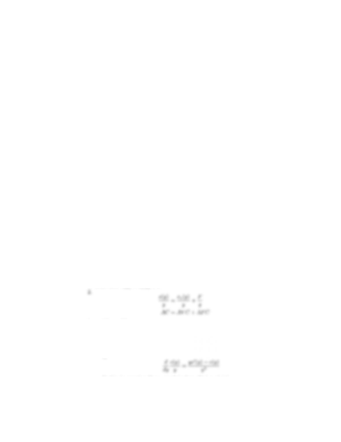
1. total cost: c(y)=cv(y)+F
3. see Figure 20.1.
4. marginal cost is the change in cost due to change in output c(y)=
dc(y)/dy =dcv(y)/dy
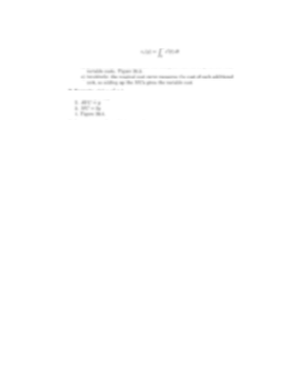
a) marginal cost equals AV C at zero units of output
b) goes through minimum point of AC and AV C. Figure 20.2.
1)
2) this is negative (for example) when c(y)<c(y)/y


