Chapter 14 NAME
Consumer’s Surplus
Introduction. In this chapter you will study ways to measure a con-
sumer’s valuation of a good given the consumer’s demand curve for it.
The basic logic is as follows: The height of the demand curve measures
how much the consumer is willing to pay for the last unit of the good
purchased—the willingness to pay for the marginal unit. Therefore the
sum of the willingnesses-to-pay for each unit gives us the total willingness
to pay for the consumption of the good.
In geometric terms, the total willingness to pay to consume some
amount of the good is just the area under the demand curve up to that
amount. This area is called gross consumer’s surplus or total benefit
of the consumption of the good. If the consumer has to pay some amount
in order to purchase the good, then we must subtract this expenditure in
order to calculate the (net) consumer’s surplus.
When the utility function takes the quasilinear form, u(x)+m,the
area under the demand curve measures u(x), and the area under the
demand curve minus the expenditure on the other good measures u(x)+
m. Thus in this case, consumer’s surplus serves as an exact measure of
utility, and the change in consumer’s surplus is a monetary measure of a
change in utility.
If the utility function has a different form, consumer’s surplus will not
be an exact measure of utility, but it will often be a good approximation.
However, if we want more exact measures, we can use the ideas of the
compensating variation and the equivalent variation.
Recall that the compensating variation is the amount of extra income
that the consumer would need at the new prices to be as well off as she
was facing the old prices; the equivalent variation is the amount of money
that it would be necessary to take away from the consumer at the old
prices to make her as well off as she would be, facing the new prices.
Although different in general, the change in consumer’s surplus and the
compensating and equivalent variations will be the same if preferences are
quasilinear.
In this chapter you will practice:
Example: Suppose that the inverse demand curve is given by P(q)=
100 −10qand that the consumer currently has 5 units of the good. How
much money would you have to pay him to compensate him for reducing
his consumption of the good to zero?
Answer: The inverse demand curve has a height of 100 when q=0
182 CONSUMER’S SURPLUS (Ch. 14)
the area of this trapezoid by applying the formula
Area of a trapezoid = base ×1
2(height1+height
2).
In this case we have A=5×1
2(100 + 50) = $375.
Example: Suppose now that the consumer is purchasing the 5 units at a
price of $50 per unit. If you require him to reduce his purchases to zero,
how much money would be necessary to compensate him?
Example: Suppose that a consumer has a utility function u(x1,x
2)=
x1+x2. Initially the consumer faces prices (1,2) and has income 10.
If the prices change to (4,2), calculate the compensating and equivalent
variations.
Answer: Since the two goods are perfect substitutes, the consumer
will initially consume the bundle (10,0) and get a utility of 10. After the
14.1 (0) Sir Plus consumes mead, and his demand function for tankards
of mead is given by D(p) = 100 −p,wherepis the price of mead in
shillings.
(a) If the price of mead is 50 shillings per tankard, how many tankards of
(b) How much gross consumer’s surplus does he get from this consump-
(d) What is his net consumer’s surplus from mead consumption?
14.2 (0) Here is the table of reservation prices for apartments taken
from Chapter 1:
Person = A B C D E F G H
NAME 183
(a) If the equilibrium rent for an apartment turns out to be $20, which
(b) If the equilibrium rent for an apartment turns out to be $20, what
is the consumer’s (net) surplus generated in this market for person A?
(c) If the equilibrium rent is $20, what is the total net consumers’ surplus
(d) If the equilibrium rent is $20, what is the total gross consumers’
(e) If the rent declines to $19, how much does the gross surplus increase?
(f) If the rent declines to $19, how much does the net surplus increase?
Calculus 14.3 (0) Quasimodo consumes earplugs and other things. His utility
function for earplugs xand money to spend on other goods yis given by
u(x, y) = 100x−x2
2+y.
(c) If the price of earplugs is $50, how many earplugs will he consume?
(d) If the price of earplugs is $80, how many earplugs will he consume?
(e) Suppose that Quasimodo has $4,000 in total to spend a month. What
is his total utility for earplugs and money to spend on other things if the
184 CONSUMER’S SURPLUS (Ch. 14)
(f) What is his total utility for earplugs and other things if the price of
$80.
(h) What is the change in (net) consumer’s surplus when the price changes
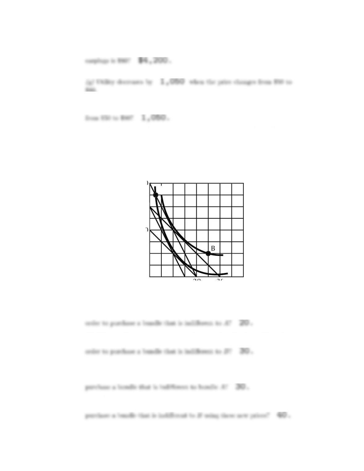
14.4 (2) In the graph below, you see a representation of Sarah Gamp’s
indifference curves between cucumbers and other goods. Suppose that
the reference price of cucumbers and the reference price of “other goods”
are both 1.
C
ucumber
s
Other goods
0
40
0
30
0
20
0
1
0
1
0
20
20
30
30
4
0
B
A
(a) What is the minimum amount of money that Sarah would need in
(b) What is the minimum amount of money that Sarah would need in
(c) Suppose that the reference price for cucumbers is 2 and the reference
price for other goods is 1. How much money does she need in order to
(d) What is the minimum amount of money that Sarah would need to
NAME 185
(e) No matter what prices Sarah faces, the amount of money she needs
to purchase a bundle indifferent to Amust be (higher, lower) than the
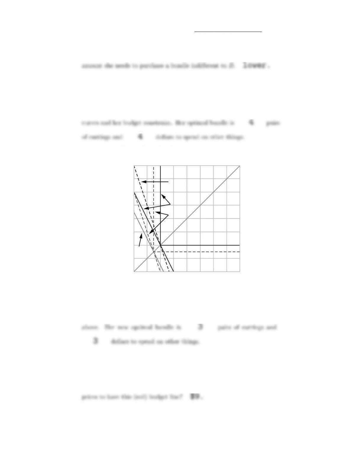
14.5 (2) Bernice’s preferences can be represented by u(x, y)=min{x, y},
where xis pairs of earrings and yis dollars to spend on other things. She
faces prices (px,p
y)=(2,1) and her income is 12.
(a) Draw in pencil on the graph below some of Bernice’s indifference
04812
16
4
8
12
Pairs of earrings
Dollars for other things
16
Black line
Pencil lines
Red
line
Blue lines
(b) The price of a pair of earrings rises to $3 and Bernice’s income stays
the same. Using blue ink, draw her new budget constraint on the graph
(c) What bundle would Bernice choose if she faced the original prices and
had just enough income to reach the new indifference curve? (3,3).
Draw with red ink the budget line that passes through this bundle at
the original prices. How much income would Bernice need at the original
186 CONSUMER’S SURPLUS (Ch. 14)
(d) The maximum amount that Bernice would pay to avoid the price
(e) What bundle would Bernice choose if she faced the new prices and had
just enough income to reach her original indifference curve? (4,4).
Draw with black ink the budget line that passes through this bundle at
the new prices. How much income would Bernice have with this budget?
(f) In order to be as well-off as she was with her original bundle, Bernice’s
Calculus 14.6 (0) Ulrich likes video games and sausages. In fact, his preferences
can be represented by u(x, y)=ln(x+1)+ywhere xis the number of
video games he plays and yis the number of dollars that he spends on
sausages. Let pxbe the price of a video game and mbe his income.
(a) Write an expression that says that Ulrich’s marginal rate of substi-
tution equals the price ratio. ( Hint: Remember Donald Fribble from
equation alone to get his demand function for video games, which is
(c) Video games cost $.25 and Ulrich’s income is $10. Then Ulrich de-
places.)
(d) If we took away all of Ulrich’s video games, how much money would
he need to have to spend on sausages to be just as well-off as before?
NAME 187
(e) Now an amusement tax of $.25 is put on video games and is passed
on in full to consumers. With the tax in place, Ulrich demands 1
(f) Now if we took away all of Ulrich’s video games, how much money
would he have to have to spend on sausages to be just as well-off as with
(g) What is the change in Ulrich’s consumer surplus due to the tax?
Calculus 14.7 (1) Lolita, an intelligent and charming Holstein cow, consumes
only two goods, cow feed (made of ground corn and oats) and hay. Her
preferences are represented by the utility function U(x, y)=x−x2/2+y,
where xis her consumption of cow feed and yis her consumption of hay.
Lolita has been instructed in the mysteries of budgets and optimization
and always maximizes her utility subject to her budget constraint. Lolita
has an income of $mthat she is allowed to spend as she wishes on cow
feed and hay. The price of hay is always $1, and the price of cow feed will
be denoted by p,where0<p≤1.
(a) Write Lolita’s inverse demand function for cow feed. (Hint: Lolita’s
utility function is quasilinear. When yis the numeraire and the price of
xis p, the inverse demand function for someone with quasilinear utility
(b) If the price of cow feed is pand her income is m,howmuchhaydoes
Lolita choose? (Hint: The money that she doesn’t spend on feed is used
(c) Plug these numbers into her utility function to find out the utility level
(d) Suppose that Lolita’s daily income is $3 and that the price of feed is
188 CONSUMER’S SURPLUS (Ch. 14)
(e) How much money would Lolita be willing to pay to avoid having the
(f) Suppose that the price of cow feed rose to $1. How much extra money
would you have to pay Lolita to make her as well-off as she was at the
(g) At the price $.50 and income $3, how much (net) consumer’s surplus
14.8 (2) F. Flintstone has quasilinear preferences and his inverse demand
function for Brontosaurus Burgers is P(b)=30−2b. Mr. Flintstone is
currently consuming 10 burgers at a price of 10 dollars.
(a) How much money would he be willing to pay to have this amount
(b) The town of Bedrock, the only supplier of Brontosaurus Burgers,
decides to raise the price from $10 a burger to $14 a burger. What
14.9 (1) Karl Kapitalist is willing to produce p/2−20 chairs at every
price, p>40. At prices below 40, he will produce nothing. If the price
of chairs is $100, Karl will produce 30 chairs. At this price, how
much is his producer’s surplus? 1
14.10 (2) Ms. Q. Moto loves to ring the church bells for up to 10
hours a day. Where mis expenditure on other goods, and xis hours of
bell ringing, her utility is u(m, x)=m+3xfor x≤10. If x>10, she
develops painful blisters and is worse off than if she didn’t ring the bells.
NAME 189
Her income is equal to $100 and the sexton allows her to ring the bell for
10 hours.
(a) Due to complaints from the villagers, the sexton has decided to restrict
Ms. Moto to 5 hours of bell ringing per day. This is bad news for Ms.
income.
(b) The sexton relents and offers to let her ring the bells as much as she
likes so long as she pays $2 per hour for the privilege. How much ringing
(c) The villagers continue to complain. The sexton raises the price of
bell ringing to $4 an hour. How much ringing does she do now? 0