Unlock document.
This document is partially blurred.
Unlock all pages and 1 million more documents.
Get Access

Chapter 14 35
Chapter 14
Consumer’s Surplus
This chapter derives consumer’s surplus using the demand theory for discrete
goods that was developed earlier in Chapters 5 and 6. I review this material in
Section 14.1 just to be safe. Given that derivation, it is easy to work backwards
to get utility.
Later in the chapter I introduce the idea of compensating and equivalent
variation. In my treatment, I use the example of a tax, but another example
that is somewhat closer to home is the idea of cost-of-living indexes for various
places to live. Take an example of an executive in New York who is offered a job
in Tucson. Relative prices differ drastically in these two locations. How much
money would the executive need at the Tucson prices to make him as well off
as he was in New York? How much money would his New York company have
to pay him to make him as well off in New York as he would be if he moved to
Tucson?
The example right before Section 14.9 shows that the compensating and the
equivalent variation are the same in the case of quasilinear utility. Finally the
appendix to this chapter gives a calculus treatment of consumer’s surplus, along
with some calculations for a few special demand functions and a numerical com-
parison of consumer’s surplus, compensating variation, and equivalent variation.
Consumer’s Surplus
A. Basic idea of consumer’s surplus
1. want a measure of how much a person is willing to pay for something. How
much a person is willing to sacrifice of one thing to get something else.
36 Chapter Highlights
B. Discrete demand
1. remember that the reservation prices measure the “marginal utility”
2. r1=v(1) −v(0), r2=v(2) −v(1), r3=v(3) −v(2), etc.
C. Continuous demand. Figure 14.2.
1. suppose utility has form v(x)+y
2. then inverse demand curve has form p(x)=v(x)
D. Change in consumer’s surplus. Figure 14.3.
E. Producer’s surplus — area above supply curve. Change in producer’s surplus
F. This all works fine in the case of quasilinear utility, but what do you do in
general?
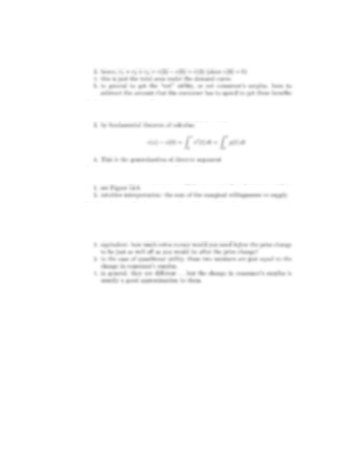
G. Compensating and equivalent variation. See Figure 14.4.
1. compensating: how much extra money would you need after a price change
to be as well off as you were before the price change?
38 Chapter Highlights
E. Elasticity
1. measures responsiveness of demand to price
2.
dq
3. example for linear demand curve
4. suppose demand takes form q=Ap−b
5. then elasticity is given by
=−p
6. thus elasticity is constant along this demand curve
F. How does revenue change when you change price?
1. R=pq,soΔR=(p+dp)(q+dq)−pq =pdq +qdp +dpdq
G. How does revenue change as you change quantity?
1. marginal revenue = MR =dR/dq =p+qdp/dq=p[1 + 1/].
2. elastic: absolute value of elasticity greater than 1
H. Marginal revenue curve
1. always the case that dR/dq =p+qdp/dq.
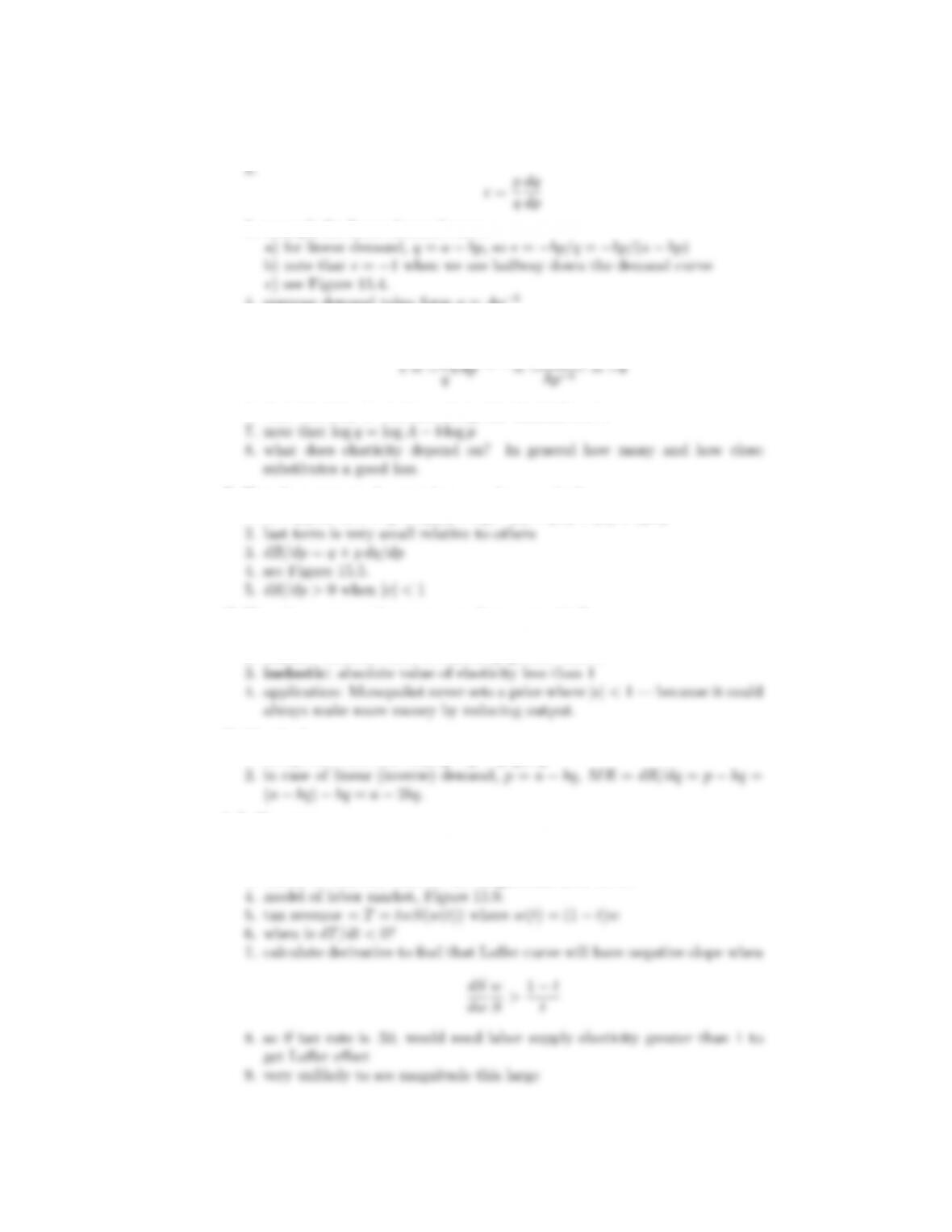
I. Laffer curve
1. how does tax revenue respond to changes in tax rates?
2. idea of Laffer curve: Figure 15.8.
3. theory is OK, but what do the magnitudes have to be?


