
157
© Pearson Education Limited 2008
Operating and Financial Leverage
It does not do to leave a live dragon out of your
calculations, if you live near him.
J.R.R. TOLKIEN, THE HOBBIT
Chapter 16: Operating and Financial Leverage
158
© Pearson Education Limited 2008
ANSWERS TO QUESTIONS
1. Operating Leverage is the use of fixed operating costs associated with the production of
goods or services. The degree of operating leverage (DOL) is the percentage change in a
2. a. Fixed; b. Variable; c. Variable;
d. Fixed – but, variable at management’s discretion;
3. Students may find Eqs. (16-3) and (16-4) of help in explaining the probable effect of a
change in a firm’s operations on the break-even point. Of course, an increase in any cost
will raise the break-even point.
a. Lower the break-even point.
5. No, this is not always the case. It is true that the presence of fixed operating costs will cause
6. You can have a high DOL and still have low business risk if sales and the production cost
7. Financial leverage is the use of fixed cost financing. The degree of financial leverage
(DFL) is the percentage change in the firm’s earnings per share (EPS) resulting from a 1
Van Horne and Wachowicz, Fundamentals of Financial Management, 13th edition, Instructor’s Manual
159
© Pearson Education Limited 2008
8. Both operating and financial leverage involve the use of fixed costs. The former is due to
fixed operating costs associated with the production of goods or services, while the latter is
10. The objective of business firms is not to maximize EPS. It is to maximize shareholder’s
11. An electric utility has much higher fixed costs in a relative sense than does the typical
manufacturing company. Also, its revenues are much more stable and predictable. Despite a
12. Whether or not, the debt-to-equity ratio is a good proxy for the cash flow ability of the firm
to service debt depends on the situation. There should be a rough correspondence between
13. The chapter has provided analytical tools to evaluate the financial structure of the firm. The
EBIT-EPS chart, cash flow available to service debt, comparison of debt ratios to industry
14. Coverage ratios should be compared with those of other companies in similar lines of
business. Where significant deviations occur, the reasons should be carefully explored. If
the average coverage ratio for the industry is used as a target, the firm could determine the
15. While earnings per share will increase as long as the firm is able to earn more on the
employment of the funds than their interest or preferred-dividend cost, risk to the common
Chapter 16: Operating and Financial Leverage
160
© Pearson Education Limited 2008
16. An increase in the debt of a company will increase the amount of periodic interest and
principal payments. The additional cash obligation for each increment in debt can be
17. Most companies are concerned with the effect a debt decision will have on its bond ratings,
both for prestige reasons and because of the interest rate they will have to pay on
borrowings. Moreover, if a rating is lowered below Baa, the company’s bonds no longer are
SOLUTIONS TO PROBLEMS
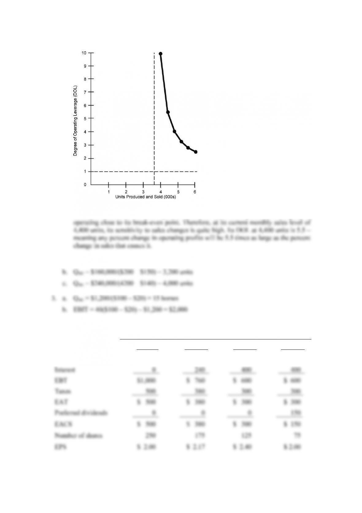
1. a. Q = $880,000/$200 = 4,400 units
b. QBE = $180,000/($200 –$150) = 3,600 units
c. DOL4,000 units = 4,000/(4,000 – 3,600) = 10.0
Van Horne and Wachowicz, Fundamentals of Financial Management, 13th edition, Instructor’s Manual
161
© Pearson Education Limited 2008
d. The graph shows that the sensitivity of a firm’s operating profit to changes in sales
decreases further, as the firm operates above its break-even point. The company is
2. a. QBE = $180,000/($250 – $150) = 1,800 units
4. a. Using an expected level of EBIT of $1 million, the earnings per share are:
Plan
1 2 3 4
EBIT (in thousands) $1,000 $1,000 $1,000 $1,000
Chapter 16: Operating and Financial Leverage
162
© Pearson Education Limited 2008
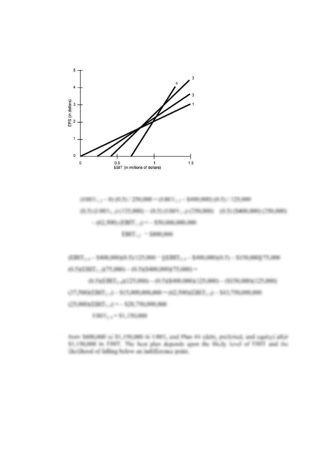
The intercepts on the horizontal axis for the four plans are $0, $240,000, $400,000, and
$700,000 respectively. With this information, the EBIT-EPS indifference chart is:
b. The “dominant” financing plans are #1, #3, and #4. For the EBIT indifference point
between Plans #1 and #3, we have:
For the indifference point between Plans #3 and #4, we have:
c. Plan #1 (all equity) dominates up to $800,000 in EBIT, Plan #3 (half debt, half equity)
Van Horne and Wachowicz, Fundamentals of Financial Management, 13th edition, Instructor’s Manual
163
© Pearson Education Limited 2008
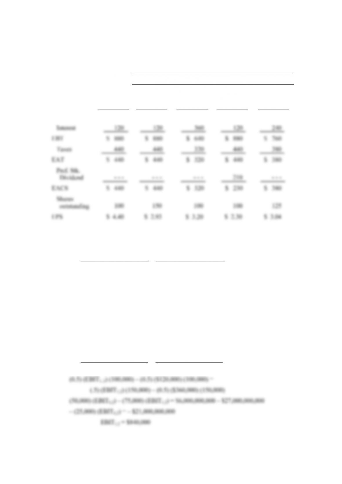
5. a. (000s omitted)
Additional-financing Plans
(1) (2) (3) (4)
Present
Capital
Structure
All
Common
All
8% Bonds
All
Preferred
Half
Common and
Half Bonds
EBIT $1,000 $1,000 $1,000 $1,000 $1,000
b. The important thing in graphing the alternatives is to include the $120,000 in interest on
existing bonds in all of the additional-financing plans. The mathematical formula for
determining the indifference point is:
1,2 1 1 1,2 2 2
12
(EBIT I ) (1 t) PD (EBIT I ) (1 t) PD
NS NS
=
––– – ––
where EBIT1, 2 = the EBIT indifference point between the two alternative financing
methods that we are concerned with – in this case, methods 1 and 2;
I1, I2 = annual interest paid under financing methods 1 and 2;
PD1, PD2 = annual preferred stock dividend paid under financing methods 1 and 2;
t = corporate tax rate;
NS1, NS2 = number of shares of common stock to be outstanding
under financing methods 1 and 2;
Comparing Plan #1 (all common) with Plan #2 (all bonds), we have:
1,2 1,2
(EBIT – $120,000) (0.5) (EBIT – $360,000) (0.5)
=
150,000 100,000
Chapter 16: Operating and Financial Leverage
164
© Pearson Education Limited 2008
Above $840,000 in EBIT, debt is more favorable (in terms of EPS); below $840,000 in
EBIT, common is more favorable.
Comparing Plan #1 (all common) with Plan #3 (all preferred), we have:
1,3 1,3
(EBIT $120,000) (0.5) (EBIT $120,000) (0.5) $210,000
=
150,000 100,000
–––
Above $1,380,000 in EBIT, Plan #3 (all preferred) is more favorable (in terms of EPS);
below $1,380,000 in EBIT, Plan #1 (all common) is more favorable.
Comparing Plan #1 (all common) with Plan #4 (half common, half bonds) we have:
1,4 1,4
(EBIT – $120,000) (0.5) (EBIT – $240,000) (0.5)
=
150,000 125,000
Above $840,000 in EBIT, Plan #4 (half common, half bonds) is more favorable (in
terms of EPS); below $840,000 in EBIT, Plan #1 (all common) is more favorable.
For the Plan #2 (all bonds) versus Plan #3 (all preferred) comparison, the bond
alternative dominates the preferred alternative by $0.90 per share throughout all levels
of EBIT.
For the Plan #2 (all bonds) versus Plan #4 (half common, half bonds) comparison, the
indifference point is again $840,000 in, EBIT.
Van Horne and Wachowicz, Fundamentals of Financial Management, 13th edition, Instructor’s Manual
165
© Pearson Education Limited 2008
For the Plan #3 (all preferred) versus Plan #4 (half common, half bonds) comparison,
we have:
These exact indifference points can be used to check graph approximations.
6. a. The level of expected EBIT is only moderately above the indifference point of
$840,000. Moreover, the variance of possible outcomes is great and there is
Looking at a normal distribution table, found in any statistics text, we find that this
corresponds to a 34.5 percent probability that the actual EBIT will be below $840,000.
b. Here the level of expected EBIT is significantly above the indifference point and the
The probability of actual EBIT falling below the indifference point is negligible. The
situation in this case favors the “all bond” alternative.