
134
© Pearson Education Limited 2008
Risk and Managerial (Real) Options in Capital
Budgeting
“Risk? Risk is our business. That’s what this starship
is all about. That’s why we’re aboard her!”
JAMES T. KIRK,
CAPTAIN OF THE STARSHIP ENTERPRISE
Van Horne and Wachowicz, Fundamentals of Financial Management, 13th edition, Instructor’s Manual
135
© Pearson Education Limited 2008
ANSWERS TO QUESTIONS
1. Investment projects with different risks can affect the valuation of the firm by suppliers of
capital. A project that provides a 20 percent expected return may add so much risk as to
2. The
standard deviation is a measure of the absolute dispersion of the probability
(To the extent that a distribution is skewed and a person is concerned with skewness, a
between measure might be the semi-variance. The semivariance is the variance of the
One alternative measure that is easy to use is the coefficient of variation (CV).
Mathematically, it is defined as the ratio of the standard deviation of a distribution to the
3. To standardize the dispersion of a probability distribution, one takes differences from the
expected value (mean) of the distribution and divides them by the standard deviation. The
4. For the riskless project the probability distribution would have no dispersion. It would be a
5. The coefficients of variation for the two projects are:
6. The
initial probabilities are those for outcomes in the first period. Conditional probabilities
are those for outcomes in subsequent periods and conditional on the outcome(s) in the
Chapter 14: Risk and Managerial (Real) Options in Capital Budgeting
136
© Pearson Education Limited 2008
7. The risk-free rate is used to discount future cash flows so as not to double count for risk. If a
premium for risk, particularly a large premium, is included in the discount rate, a risk
8. Simulation gives the analyst an idea of the dispersion of likely returns from a project as well
9. The greater the correlation of net present values among projects, the greater the standard
10. A portfolio of assets dominates another if it has a higher expected return and the same or
11. When a decision maker decides on a portfolio of assets, that determines the acceptance or
12. A managerial option has to do with management’s flexibility to make a decision after a
project is accepted that will alter the project’s subsequent expected cash flows and/or its
13. The present value of a managerial option is determined by the likelihood that it will be
exercised and the magnitude of the resulting cash-flow benefit. The greater the uncertainty
14. Managerial options include (i) the option to expand production in the future if things turn
out well (or to contract if conditions do not turn out well), (ii) the option to abandon a
project, and (iii) the option to postpone a project’s acceptance or launch. Options (i) and (ii)
Van Horne and Wachowicz, Fundamentals of Financial Management, 13th edition, Instructor’s Manual
137
© Pearson Education Limited 2008
SOLUTIONS TO PROBLEMS
1. a. Simply by looking, project B looks less risky.
b. E(CFA) = (0.2) ($2,000) + (0.3) ($4,000)
B clearly dominates A since it has lower risk for the same level of return.
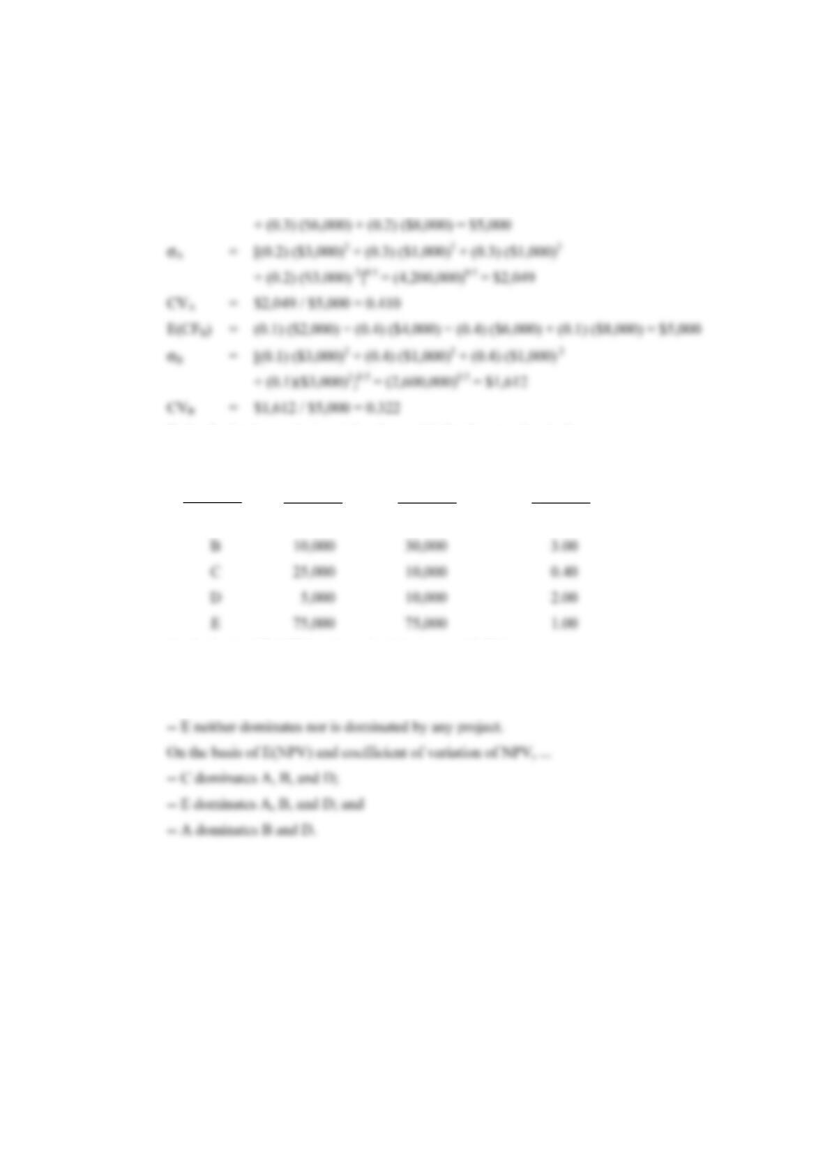
2. a.
Project E(NPV) σNPV CVNPV
A $10,000 $20,000 2.00
On the basis of E(NPV) and standard deviation of NPV, …
— C dominates A, B, and D;
— A dominates B and D; and
Chapter 14: Risk and Managerial (Real) Options in Capital Budgeting
138
© Pearson Education Limited 2008
b.
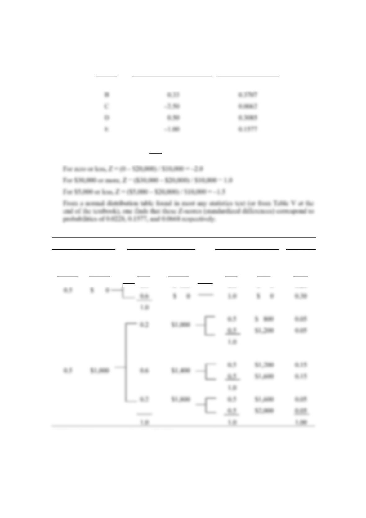
Project Z-score (0 – E(NPV))/σNPV Probability (NPV < 0)
A –0.50 0.3085
3. The general formula to use is:
Z (the Z-score) = (NPV* –
N
PV )/σNPV
4.
Year 1 Year 2 Year 3 Overall
Initial
Prob.
Net Cash
Flow
Cond.
Prob.
Net Cash
Flow
Cond.
Prob.
Net
Cash
Flow
Joint
Prob.
0.4 –$ 300 1.0 $ 0 0.20
NOTE: Initial investment at time 0 = $1,000.
Van Horne and Wachowicz, Fundamentals of Financial Management, 13th edition, Instructor’s Manual
139
© Pearson Education Limited 2008
b.
(1)
Cash Flow
Series
(2)
Net Present
Value
(3)
Joint Probability of
Occurrence
(4)
(2) × (3)
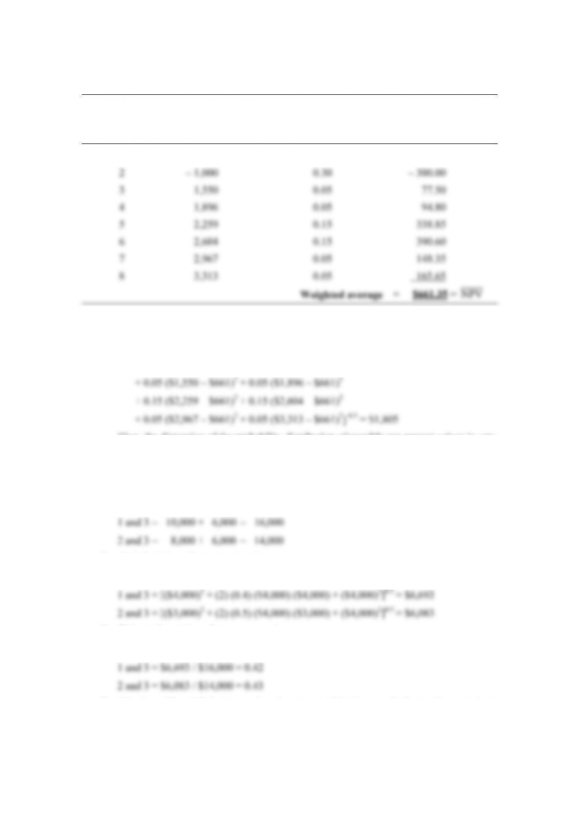
1 –$1,272 0.20 –$254.40
c. The expected value of net present value of the project is found by multiplying together
the last two columns above and totaling them. This is found to be $661 (after rounding).
d. The standard deviation is:
[0.20 (–$1,272 – $661)2 + 0.30 (–$1,000 – $661)2
Thus, the dispersion of the probability distribution of possible net present values is very
wide. In addition to the distribution being very wide, there is also a 50 percent
probability of NPV being less than zero.
5. Expected net present value:
1 and 2 = $10,000 + $8,000 = $18,000
Standard deviation of net present value:
1 and 2 = [($4,000)2 + (2) (0.6) ($4,000) ($3,000) + ($3,000)2]0.5 = $6,277
Coefficient of variation of net present value:
1 and 2 = $6,277 / $18,000 = 0.35
Combination of 1 and 2 dominates the other two combinations on the basis of expected net
present value and coefficient of variation of net present value.
Chapter 14: Risk and Managerial (Real) Options in Capital Budgeting
140
© Pearson Education Limited 2008
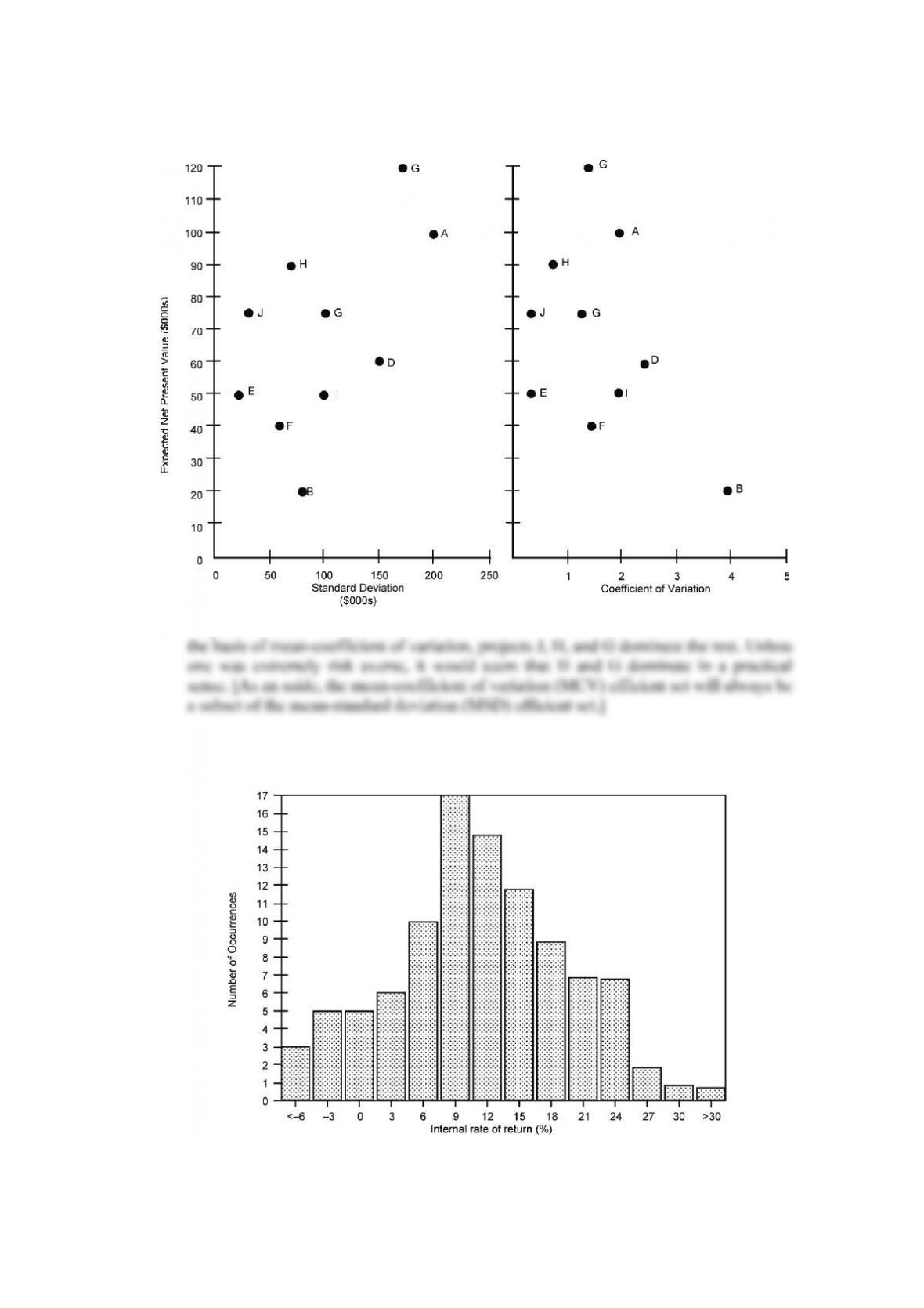
6. a.
b. Projects E, J, H, and G dominate the rest on the basis of mean-standard deviation. On
7. a. Each simulation will differ somewhat, so there is no exact answer to this problem. A
simulation involving 100 runs resulted in the following IRR distribution:
Van Horne and Wachowicz, Fundamentals of Financial Management, 13th edition, Instructor’s Manual
141
© Pearson Education Limited 2008
b. The most likely IRR was in the 7 to 9 percent range – a relatively modest return. As can
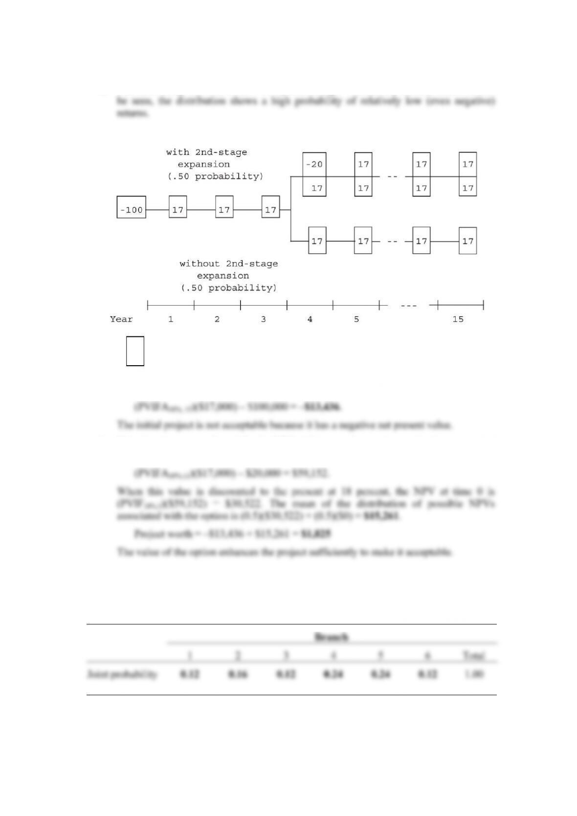
8.
Key: │ │ expected cash flows in $000s
└——┘
a. NPV of initial project at 18 percent required rate of return equals
b. If the location proves favorable, the NPV of the second-stage (expansion) investment at
the end of year 4 will be
SOLUTIONS TO SELF-CORRECTION PROBLEMS
1. a.
Chapter 14: Risk and Managerial (Real) Options in Capital Budgeting
142
© Pearson Education Limited 2008
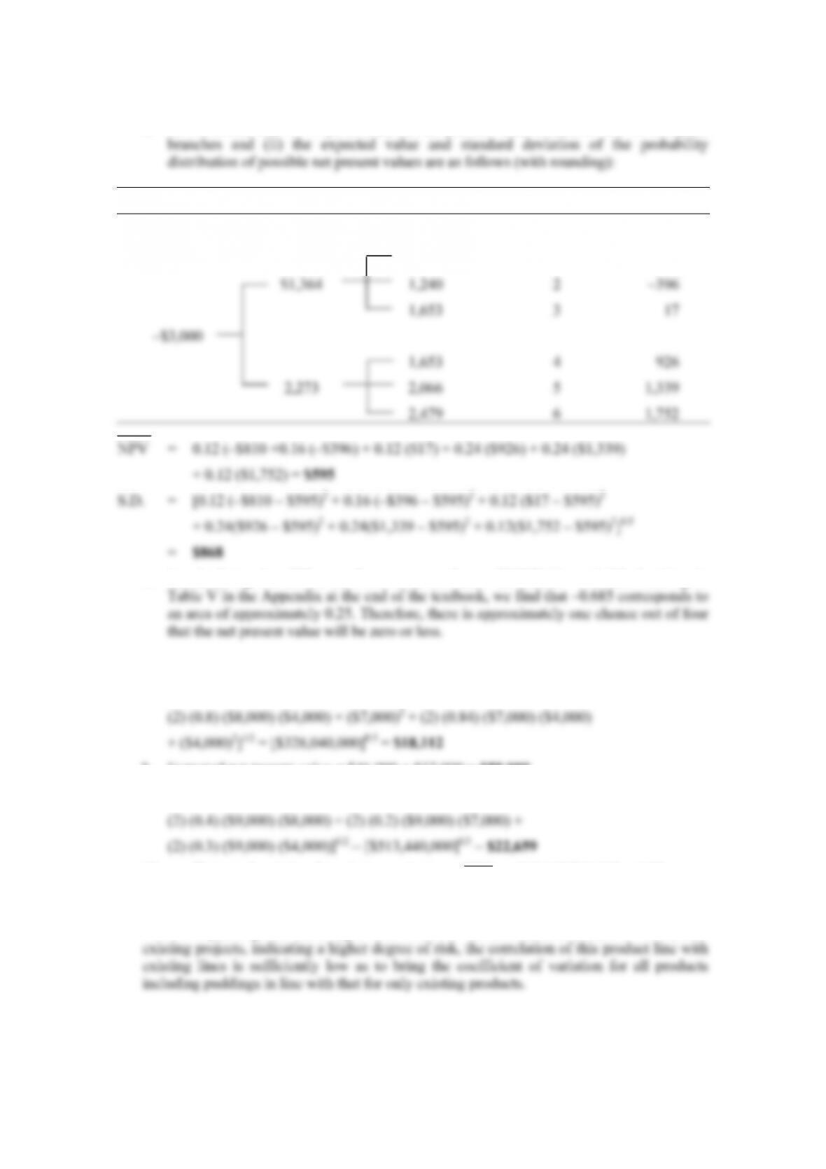
b. At a risk-free rate of 10 percent (i) the net present value of each of the six complete
Year 0 Year 1 Year 2 Branch NPV
$ 826 1 –$ 810
c. Standardizing the difference from zero, we have –$595/$868 = –0.685. Looking in
2. a. Expected net present value = $16,000 + $20,000 + $10,000 = $46,000
Standard deviation = [($8,000)2 + (2) (0.9) ($8,000) ($7,000) +
b. Expected net present value = $46,000 + $12,000 = $58,000
Standard deviation = [$328,040,000 + ($9,000)2 +
The coefficient of variation for existing projects (/NPV)
σ
= $18,112/$46,000 = 0.39.
The coefficient of variation for existing projects plus puddings = $22,659/$58,000 = 0.39.
While the pudding line has a higher coefficient of variation ($9,000/$12,000 = 0.75) than
Van Horne and Wachowicz, Fundamentals of Financial Management, 13th edition, Instructor’s Manual
143
© Pearson Education Limited 2008
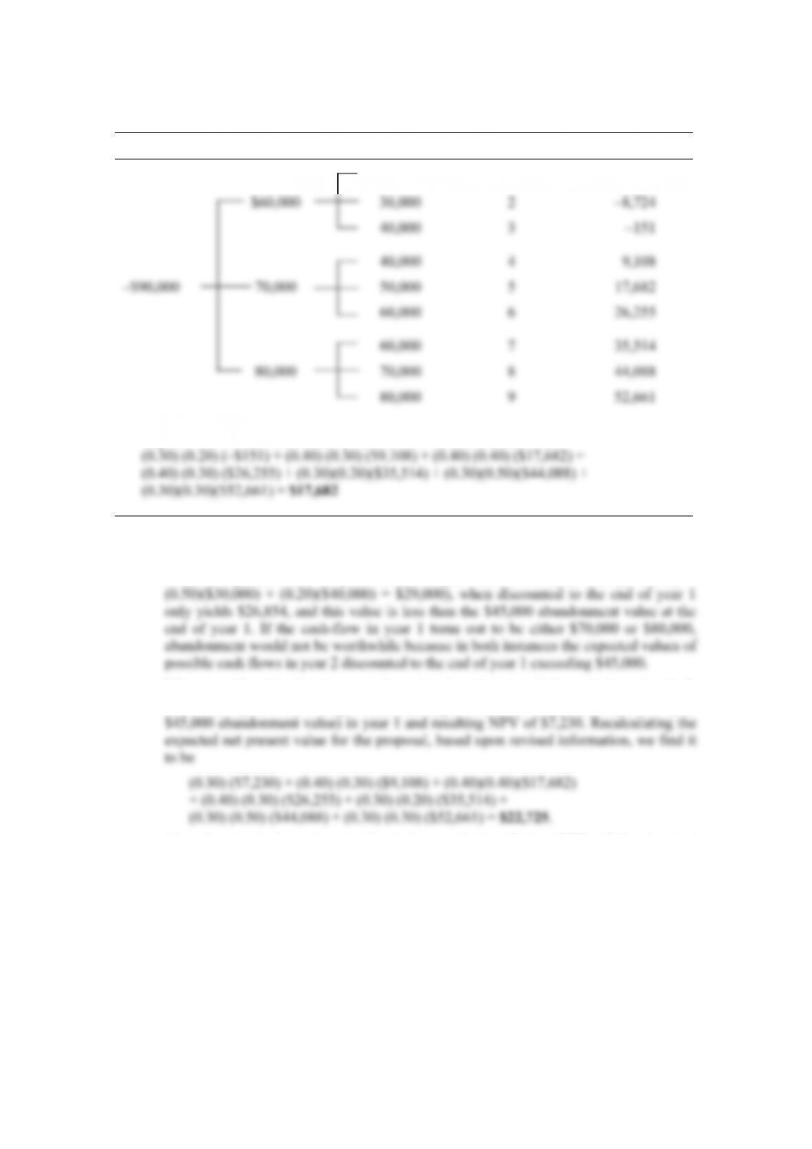
3. a.
Year 0 Year 1 Year 2 Branch NPV
$20,000 1 –$17,298
Expected NPV = (0.30) (0.30) (–$17,298) + (0.30) (0.50) (–$8,724) +
b. We should abandon the project at the end of the first year if the cash-flow in that year
turns out to be $60,000. The reason is that given a $60,000 first year cash-flow, the
$29,000 expected value of possible second-year cash flows (i.e., (0.30)($20,000) +
When we allow for abandonment, the original projected cash flows for branches 1, 2,
and 3 are replaced by a single branch having a cash-flow of $105,000 ($60,000 plus
Thus, the expected net present value is increased when the possibility of abandonment
is considered in the evaluation. Part of the downside risk is eliminated because of the
abandonment option.