
Chapter 3
1. You wish to estimate the utility to you of earning the annual salaries in the left column of
Table 3.1. You fix the utility of $10,000 arbitrarily at 15, and the utility of $40,000 arbitrarily at
25. You decide that you are indifferent between (a) receiving a sure salary of Q between $10,000
and $40,000 and (b) taking a chance of receiving $40,000 with probability p and $10,000 with
probability 1 p, where Q and p are shown in the table. Calculate the utility of salaries
$15,000, $20,000, and $30,000.
The utility u(Q) of receiving a sure salary of Q is the expected utility
(1 ) (10,000) (40,000)– +p u pu
where p is the probability for which you are indifferent between (a) receiving Q for sure and (b)
receiving 40,000 with probability p and 10,000 with probability
1 p. So
(15,000) (1 0.35) (10,000) (0.35) (40,000) (0.65)(15) (0.35)(25) 18.5= – + = + =u u u
(20,000) (1 0.6) (10,000) (0.6) (40,000) (0.4)(15) (0.6)(25) 21= – + = + =u u u
(30,000) (1 0.85) (10,000) (0.85) (40,000) (0.15)(15) (0.85)(25) 23.5= – + = + =u u u
2.* The previous exercise does not yield utilities for $5,000 and $50,000. However, you are
indifferent between (a) receiving $10,000 for sure and (b) receiving $40,000 with probability p
and $5,000 with probability 1 p, where p = 1/3. Use this to calculate the utility of $5,000.
Hint. Suppose, in general, that you fix utilities for salaries Q1 and Q2 (here, $10,000 and
$40,000, respectively) and wish to calculate the utility of some salary Q that is less than
$10,000. If you are indifferent between (a) receiving Q1 and (b) a lottery in which you receive Q2
with probability p and Q with probability 1 p, then this allows you to solve for u(Q) in terms of
u(Q1) and u(Q2).
Following the hint, we equate the utility of Q1 with the expected utility of the lottery involving Q
and Q2:
1 2
( ) (1 ) ( ) ( )= – +u Q p u Q pu Q
Solving for u(Q), we get
1 2
( ) ( ) (10,000) (1 / 3) (40,000) 15 (1/ 3)(25)
( ) = 10
1 1 (1/ 3) 2 / 3
– – –
= = =
– –
u Q pu Q u u
u Q p

3. Suppose you are indifferent between (a) receiving a salary of $40,000 for sure and (b) a
lottery in which you receive $50,000 with probability p and $10,000 with probability 1 p,
where p = 0.9. Use this fact to calculate the utility of $50,000.
Following the pattern of the previous exercise, we equate the utility of Q2 with the expected
utility of the lottery involving Q1 and Q:
2 1
( ) (1 ) ( ) ( )= – +u Q p u Q pu Q
Solving for u(Q):
1
2 1
9
( ) (1 ) ( ) (40, 000) (0.1) (10,000) 25 (0.1)(15)
( ) = 26
0.9 0.9
– – – –
= = =
u Q p u Q u u
u Q p
So the utility of 50,000 is
1
9
26
.
4. Plot your utility curve using the results of the previous three exercises.
The curve appears below.
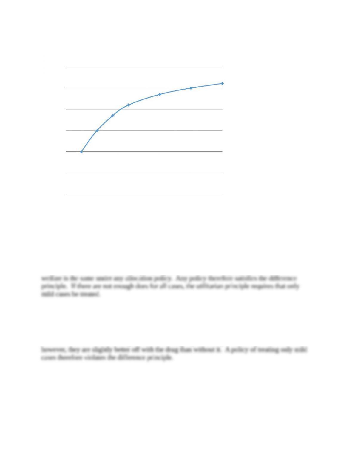
Utility Curve
Q
u(Q)
5.* A drug is discovered that cures all mild cases of diabetes but has no effect on severe cases.
It is therefore prescribed only for patients who have mild cases. Does this policy satisfy the
Difference Principle?
There are two relevant groups: patients with mild cases and those with severe cases. Patients
with severe cases are the worse-off group regardless of how the drug is prescribed, and their
6. Suppose the drug in the previous exercise cures all mild cases but has only a small positive
effect on severe cases. The drug is in short supply, and to make the best use of it, it is prescribed
only for patients with mild cases. Does this policy satisfy the Difference Principle?
Patients with severe cases are again the worse off group under any allocation policy. This time,
7. Some provincial governments conduct daily lotteries. Studies have found that those who buy
the lottery tickets are the poorest people in the province. Does this type of lottery satisfy the
difference principle?
There are two relevant groups: citizens of the province who are inclined to buy lottery tickets and
those who aren’t. The former group is worse off whether or not tickets are sold. If tickets are
8.* An economics game. A popular economics game teaches an important lesson in rationality.
You are granted $100 along with the option of donating any portion of the grant (from $0 to
$100) to an anonymous person. That person, to whom the donor is anonymous, is given the
option of accepting or rejecting the donation. If the gift is rejected, both parties forfeit the
money. No collusion is allowed. Clearly, rational self-interest requires that you donate a very
small positive amount (say, one cent) and that the recipient accept it. If you donated zero, the
recipient could reject it without penalty, but it is irrational to turn down even one cent. Actual
behavior is quite different. The average donation tends to be in the range of $30–40, and close
to half give away $50. This behavior is normally cited as a demonstration that people are
irrational. Yet this follows only if rationality is interpreted in the narrow sense of rational
self-interest. How can the observed behavior, particular the behavior of those who donate half
the money, be seen as entirely rational from a Rawlsian perspective?
If we suppose that donors and recipients are equally well off on the average before playing the
game, the donors who donate half their money follow the Rawlsian difference principle