Chapter 4 Return and Risk 65
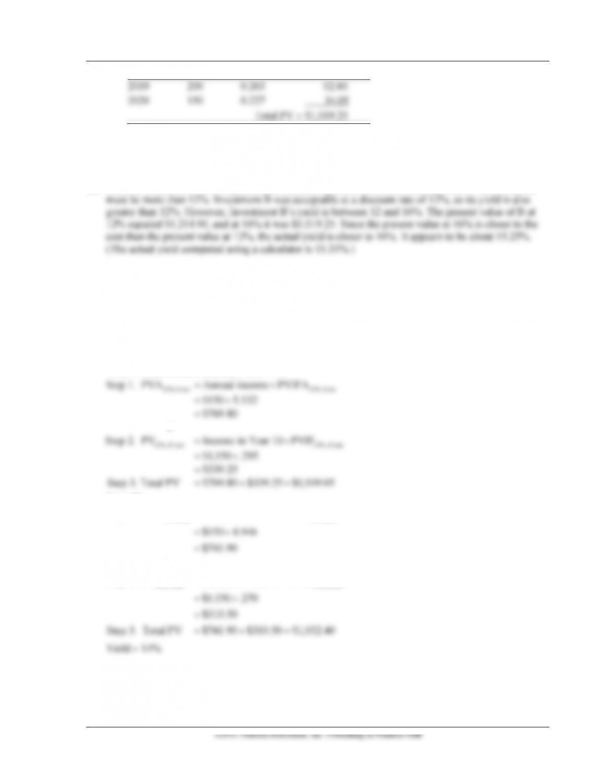
2019
200
0.263
52.60
2020
150
0.227
34.05
Total PV = $1,019.25
Since $1,019.25, the present value of Investment B, does not remain greater than its cost ($1,050), it
is no longer an acceptable investment. Investment A is the only one of the two earning a reasonable
(i.e., acceptable) return.
(c) Since Investment A was acceptable (had a positive present value) at a discount rate of 12%, its yield
(d) Investment A: Present value technique:
Step 1. Find the present value of $150 income for nine years using the present value of an annuity
formula.
Step 2. Find the PV of $1,150 in year 10.
Step 3. Add the two amounts to get the total PV. Try different discount rates to determine the yield
(IRR). Because we know from Question 1 that the present value at 12% is $1,196.50, just above the
initial investment amount, start with 13%:
=
=
=
+
=
=
=
= + =
13%, 9 yrs. 13%, 9 yrs.
13%,10 yrs. 13%,10 yrs.
Step 1. PVA Annual income PVIFA
$150 5.132
$769.80
Step 2. PV Income in Year 10 PVIF
$1,150 .295
$339.25
Step 3. Total PV $769.80 $339.25 $1,109.05
Try 14%:
=
=
=
+
=
=
=
= + =
14%, 9 yrs. 14%, 9 yrs.
14%, 10 yrs. 14%, 10 yrs.
Step 1. PVA Annual income PVIFA
$150 4.946
$741.90
Step 2. PV Income in Year 10 PVIF
$1,150 .270
$310.50
Step 3. Total PV $741.90 $310.50 $1,052.40
66 Gitman/Joehnk/Smart • Fundamentals of Investing, Eleventh Edition
Investment B: Because the present value of the income from Investment B is $1,019.25 at 16%
(Question 2), try a 15% discount rate:
(1)
(2)
(3)
(1) – (2)
Year
Benefit
15% PVIF
Present Value
2011
$100
0.870
$87.00
2012
150
0.756
113.40
2013
200
0.658
131.60
2014
250
0.572
143.00
2015
300
0.497
149.10
2016
350
0.432
151.20
2017
300
0.376
112.80
2018
250
0.327
81.75
2019
200
0.284
56.80
2020
150
0.247
37.05
Total PV = $1,063.70
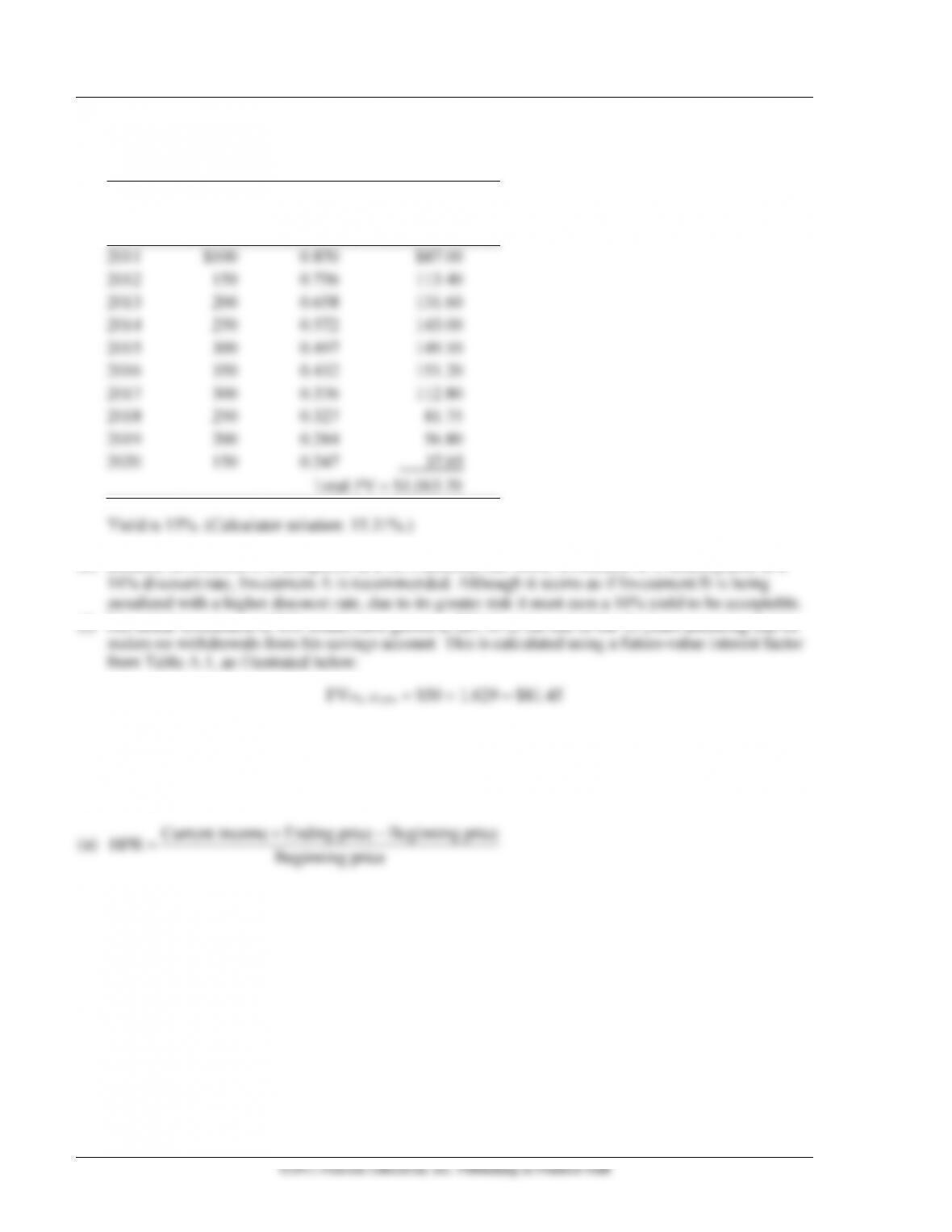
Yield is 15%. (Calculator solution: 15.31%.)
(e) Because Investment A is acceptable at a 12% discount rate while Investment B is unacceptable at a
(f) His initial investment of $50 would have grown to $81.45 at the end of the 10 years assuming that he
Case 4.2 The Risk-Return Tradeoff: Molly O’Rourke’s Stock
Purchase Decision
The title of this case clearly states its objective. It requires students to review and apply the concept of the
risk-return trade-off.
+−
©2011 Pearson Education, Inc. Publishing as Prentice Hall
(1)
(2)
(3)
(4)
(2) – (3)
(5)
[(1) + (4)]/(3)
Year
Current
Income
Ending
Price
Beginning
Price
Capital
Gain
HPR
2001
$1.00
$22.00
$20.00
$2.00
15.00%
2002
1.50
21.00
22.00
–1.00
2.27
2003
1.40
24.00
21.00
3.00
20.95
2004
1.70
22.00
24.00
–2.00
–1.25
2005
1.90
23.00
22.00
1.00
13.18
2006
1.60
26.00
23.00
3.00
20.00
2007
1.70
25.00
26.00
–1.00
2.69
2008
2.00
24.00
25.00
–1.00
4.00
2009
2.10
27.00
24.00
3.00
21.25
2010
2.20
30.00
27.00
3.00
19.26
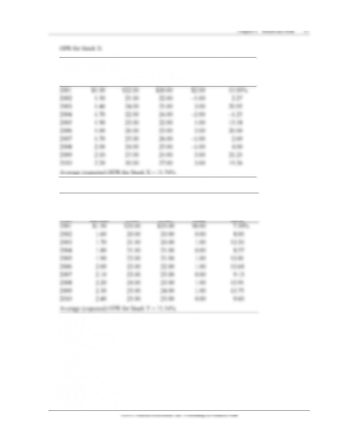
Average (expected) HPR for Stock X = 11.74%
HPR for Stock Y:
(1)
(2)
(3)
(4)
(2) – (3)
(5)
[(1) + (4)]/(3)
Year
Current
Income
Ending
Price
Beginning
Price
Capital
Gain
HPR
2001
$1.50
$20.00
$20.00
$0.00
7.50%
2002
1.60
20.00
20.00
0.00
8.00
2003
1.70
21.00
20.00
1.00
13.50
2004
1.80
21.00
21.00
0.00
8.57
2005
1.90
22.00
21.00
1.00
13.81
2006
2.00
23.00
22.00
1.00
13.64
2007
2.10
23.00
23.00
0.00
9.13
2008
2.20
24.00
23.00
1.00
13.91
2009
2.30
25.00
24.00
1.00
13.75
2010
2.40
25.00
25.00
0.00
9.60
Average (expected) HPR for Stock Y = 11.14%
68 Gitman/Joehnk/Smart • Fundamentals of Investing, Eleventh Edition
©2011 Pearson Education, Inc. Publishing as Prentice Hall
(b)
2
1
()
1
n
i
i
rr
s
N
=
−
=−
Investment X:
(1)
(2)
(3)
(4)
Return
Average
(1) – (2)
(3)2
Year
ri
Return, r
ri – r
(ri – r)2
2001
15.00%
11.74%
3.26%
10.63%
2002
2.27
11.74
–9.47
89.68
2003
0.95
11.74
9.21
84.82
2004
–1.25
11.74
–12.99
168.74
2005
13.18
11.74
1.44
2.07
2006
20.00
11.74
8.26
68.23
2007
2.69
11.74
–9.05
81.90
2008
4.00
11.74
–7.74
59.91
2009
21.25
11.74
9.51
90.44
2010
19.26
11.74
7.52
56.55
712.97
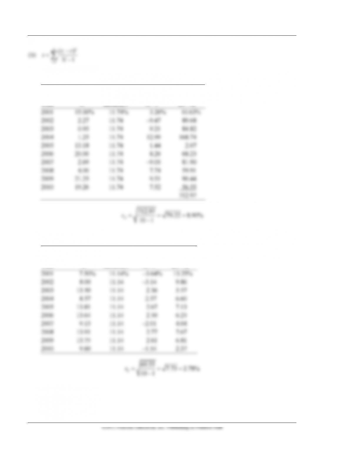
= = =
−
712.97 79.22 8.90%
10 1
X
s
Investment Y:
(1)
(2)
(3)
(4)
Return
Average
(1) – (2)
(3)2
Year
ri
Return, r
ri – r
(ri – r)2
2001
7.50%
11.14%
–3.64%
13.25%
2002
8.00
11.14
–3.14
9.86
2003
13.50
11.14
2.36
5.57
2004
8.57
11.14
–2.57
6.60
2005
13.81
11.14
2.67
7.13
2006
13.64
11.14
2.50
6.25
2007
9.13
11.14
–2.01
4.04
2008
13.91
11.14
2.77
7.67
2009
13.75
11.14
2.61
6.81
2010
9.60
11.14
–1.54
2.37
69.55 7.73 2.78%
10 1
Y
s= = =
−
Chapter 4 Return and Risk 69
(c) and (d)
Summary statistics:
Investment X
Investment Y
Expected Return
11.74%
11.14%
Standard Deviation
8.82
2.78
Comparing the expected returns calculated in Question 1, Stock X provides a return of 11.74%,
which is only slightly above the expected return of Y (11.14%). Whether the higher return on
Stock X is sufficient to compensate for the higher risk would be determined by the “price of risk” in
the financial markets.
As can be seen, standard deviation of Stock X is higher than the corresponding values of Stock Y.
This might be a signal to prefer Stock Y. But these numbers have to be interpreted with caution, as
one of the above stocks is to be added to a well-diversified portfolio.
This part of the case problem anticipates the use of beta and the capital asset pricing model (CAPM),
which will be covered in the next chapter on modern portfolio concepts. The calculation of required
return provides an objective approach to assess the investment risk.
Using the capital asset pricing model, the required return on each stock is as follows:
Investment
r
Rf + [bI (rm − RF)]
A
11.8% = 7% + [1.6 (10% − 7%)]
B
10.3% = 7% + [1.1 (10% − 7%)]
From the calculations in Question 1, Stock X has an expected return of 11.74% and a required return
of 11.80%. On the other hand, Stock Y has an expected return of 11.14% and a required return of
only 10.30%.
So while we concluded that it would be difficult to make a choice between X and Y because the
additional return on X may or may not provide the needed compensation for the extra risk, we see
that by calculating a required rate of return, it is easy to reject X and invest in Y. The required

70 Gitman/Joehnk/Smart • Fundamentals of Investing, Eleventh Edition
Appendix: The Time Value of Money
◼ Outline
4A-I. Interest: The Basic Return to Savers
4A-II. Simple Interest
4A-III. Compound Interest
4A-IV. Computational Aids for Use in Time Value Calculations
A. Financial Calculators
B. Computers and Spreadsheets
4A-V. Future Value: An Extension of Compounding
A. Calculator Use
B. Spreadsheet Use
4A-VI. Present Value: An Extension of Future Value
A. Calculator Use
B. Spreadsheet Use
4A-VII. Present Value of a Stream of Returns
A. Present Value of a Mixed Stream
1. Calculator Use
2. Spreadsheet Use
B. Present Value of an Annuity
1. Calculator Use
2. Spreadsheet Use
Concepts in Review
◼ Overview
The vitally important concepts of the time value of money, future value, and present value are covered in
an appendix to Chapter 4. These concepts are best explained by working through a few examples that deal
with single sums, annuities, and mixed streams. The instructor should emphasize that present value
calculations provide a dollar value (in today’s terms) of future cash flows. The present value concept is a
powerful tool that makes it possible to compute the dollar value of any asset. Some assets that might be
profitably considered in class are stocks, bonds, other financial assets, physical assets (machines), real
estate, and even companies themselves.
Chapter 4 Return and Risk 71
◼ Answers to Concepts in Review
4A.1. Time value of money refers to the fact that, with the opportunity to earn interest on funds, the value
of money depends on the point in time when the money is expected to be received. Thus, the
4A.2. (a) Interest is the income you receive from placing available funds in a savings account, CD,
bond, or by making a loan. It is in effect the “rent” paid on your money by those who obtain
4A.3. The true rate of interest rises, as interest is compounded more frequently than annually. The true
4A.4. The future value of a cash flow represents the amount to which a current deposit will grow over a
4A.5. An annuity is a stream of equal cash flows that occur in equal intervals over time. These cash
72 Gitman/Joehnk/Smart • Fundamentals of Investing, Eleventh Edition
4A.6 A mixed stream of returns is a series of returns that exhibits no pattern. To find the present value
◼ Solutions to Problems
4A-1. The simple interest calculations for parts (a) and (b) can be presented in tabular form:
(b)
(a)
Date
Beginning
Balance*
Annual
Interest
Ending
Balance**
1/1/11
$5,000
$5,000 .06 = $300
$5,000
1/1/12
1,000
1,000 .06 = 60
1,000
1/1/13
3,000
3,000 .06 = 180
3,000
1/1/14
6,000
6,000 .06 = 360
6,000
Assuming all transactions occur at the beginning of the period
Since all interest earned is withdrawn, the ending account balance equals the
beginning account balance.
4A.2. (a) Future value of $300 in 12 years at 7% annual compound interest:
=
=
=
=
Future value Present value Future-value interest factor
$300 (FVIF, 12 years, 7%)
$300 (2.252)*
$675.60
* From Table A.1, Appendix A.
(b) The future value at the end of six years of an $800 annual end-of–year deposit at 7% interest:
=
=
=
=
Future value Deposit Future-value interest factor for an annuity
FV $800 (FVIF, 6 years, 7%)
$800 (7.153)*
$5,722.40
* From Table A.2, Appendix A.
Note: For simplicity, the problems in the rest of the chapter use the abbreviations FV, FVIF, FVIFA, PV,
PVIF, PVIFA, and k (interest rate/rate of return), n (number of years/investment period).
Chapter 4 Return and Risk 73
4A.3. Future value of an investment: FVn = Investment amount FVIFk, n
Investment
A
FV20 = PV FVIF5%, 20 yrs.
FV20 = $200 2.653
FV20 = $530.60
Calculator solution: $530.66
B
FV7 = PV FVIF8%, 7 yrs.
FV7 = $4,500 1.714
FV7 = $7,713
Calculator solution: $7,712.21
C
FV10 = PV FVIF9%, 10 yrs.
FV10 = $10,000 2.367
FV10 = $23,670
Calculator solution: $23,673.64
D
FV12 = PV FVIF10%, 12 yrs.
FV12 = $25,000 3.138
FV12 = $78,450
Calculator solution: $78,460.71
E
FV5 = PV FVIF11%, 5 yrs.
FV5 = $37,000 1.685
FV5 = $62,345
Calculator solution: $62,347.15
4A.4. This is a future value equation. Calculate the future value of $10,000 using a FVIF1%, 24 periods value.
$10,000 1.270 = $12,700.
4A.5. Future value of an annuity investment: FVAk, n = Annual deposit FVIFAk, n
Investment
A
FVA8%, 10 yrs.
= $2,500 14.487
= $36,217.50
Calc. Sol’n.
= $36,216.41
B
FVA12%, 6 yrs.
= $500 8.115
= $4,057.50
Calc. Sol’n.
= $4,057.59
C
FVA20%, 5 yrs.
= $1,000 7.442
= $7,442
Calc. Sol’n.
= $7,441.60
D
FVA6%, 8 yrs.
= $12,000 9.897
= $118,764
Calc. Sol’n.
= $118,769.61
E
FVA14%, 30 yrs.
= $4,000 356.778
= $1,427,112
Calc. Sol’n.
= $1,427,147.39
FVIFA from Appendix A, Table A.2.
74 Gitman/Joehnk/Smart • Fundamentals of Investing, Eleventh Edition
©2011 Pearson Education, Inc. Publishing as Prentice Hall
4A.6. Future value of an annuity of $1,000 for five years at 6%. $1,000 5.637 = $5,637.
4A.7. The least you would accept for each investment is its future value at the end of six years:
(a) Future value of an investment: FVn = Investment amount FVIFk, n
=
9%, 6 yrs
FV $5,000 1.677
(b) Future value of an annuity investment:
=
,,
FVA Annual deposit FVIFA
k n k n
=
9%, 6 yrs.
FVA $2,000 7.523
(c) FV of $3,000 at 9% for six years + FVA of $1,000 deposit at 9% at end of each of the next
five years:
(2) FVA9%, 6 yrs. = $1,000 7.523 (from App. A, Table A.2)
(3) Total = $5,031 + $7,523
(d)
Year
End-of-Year
Deposit
Number
of Years
to Compound
FVIF, 9%
Future
Value
1
$900
5
1.539
$1,385.10
3
900
3
1.295
1,165.50
5
900
1
1.090
981.00
Total FV =
$3,531.60
4A.8. Present value: PV = FVn PVIFk, n
Investment
FV PVIF
Present
Value
Calculator
Solution
A
PV12%, 4 yrs.* = $7,000 .636
=
$4,452
$4,448.63
B
PV8%, 20 yrs.* = $28,000
.215
=
$6,020
$6,007.35
C
PV14%, 12yrs.* = $10,000
.208
=
$2,080
$2,075.59
D
PV11%, 6yrs. = $150,000
.535
=
$80,250
$80,196.13
E
PV20%, 8yrs = $45,000 .233
=
$10,485
$10,465.56
PVIF from Table A.3, Appendix A.
76 Gitman/Joehnk/Smart • Fundamentals of Investing, Eleventh Edition
4A.13. (a)
Income
Stream
End of
Year
Income 15% PVIF
Present
Value
A
1
$4,000 .870
=
$3,480
2
3,000 .756
=
2,268
3
2,000 .658
=
1,316
4
1,000 .572
=
572
$7,636
Calculator solution =
$7,633.48
B
1
$1,000 .870
=
$870
2
2,000 .756
=
1,512
3
3,000 .658
=
1,974
4
4,000 .572
=
2,288
$6,644
Calculator solution =
$6,641.41
PVIF from Table A.3, Appendix A.
(b) Income Stream A, with a present value of $7,636, is higher than Income Stream B’s present
4A.14. The present value of an investment with annual income streams is calculated using the formula:
PVAn = Annual returns PVIFAk, n
Investment
Calculation
Present Value
Calc. Sol’n
A
PVA7%, 3 yrs.
=
$1,200 2.624
=
$3,148.80
$3,149.18
B
PVA12%, 15 yrs.
=
5,500 6.811
=
37,460.50
37,459.75
C
PVA20%, 9 yrs.
=
700 4.031
=
2,821.70
2,821.68
D
PVA5%, 7 yrs.
=
14,000 5.786
=
81,004.00
81,009.23
E
PVA10%, 5 yrs.
=
2,200 3.791
=
8,340.20
8,339.73
4A.15. Find the present value of the annuity and compare it to the lump sum payment.
4A.16. (a) Present value of $500 to be received in four years at an 11% discount rate:
=
=
=
11%, 4yrs.
PV FV PVIF
$500 .659
$329.50
PVIF from Table A.3, Appendix A.
(b) The present value of the income from Stream A is the present value of an annuity.
9%,7 yrs.
Stream A
PVA Annual income PVIFA
PVA $80 (5.033)
$402.64
=
=
=
PVIFA from Table A.4, Appendix A.
Chapter 4 Return and Risk 77
The present value at the start of 2006 of the income from Stream B is the present value of a
mixed stream—the present value of each benefit summed.
(1)
(2)
(3)
(1) (2)
Year
Benefit
PVIF, 9%
Present Value
2012
$140
0.917
$128.38
2013
120
0.842
101.04
2014
100
0.772
77.20
2015
80
0.708
56.64
2016
60
0.650
39.00
2017
40
0.596
23.84
2018
20
0.547
10.94
Total
$437.04
PVIF from Table A.3, Appendix A.
Note: These streams may be used to illustrate the time value of money. Both streams have $560
in total benefits, but the benefits in Stream A are presently worth $402.64, while the benefits in
Stream B are worth $437.04. The difference is attributable to the fact that Stream B has larger
benefits or cash flows earlier, thereby causing its present value at the 9% rate to be higher than
Stream A.
4A.17. The analysis of Terri’s investment opportunities uses the formula: FVn = PV FVIFk, n
Investment
Calculation
Decision
A
$30,000 = $18,000 FVIFk,
5yrs.
=, 5 yrs.
$30,000 FVIF
$18,000 k
1.667 = FVIFk, 5 yrs.
10% < k < 11%
Invest
B
$3,000 = $600 FVIFk, 20 yrs.
=, 20 yrs.
$3,000 FVIF
$600 k
5 = FVIFk, 20 yrs.
8% < k < 9%
Forgo
C
$10,000 = $3,500 FVIFk, 10
yrs.
=, 10 yrs.
$10,000 FVIF
$3,500 k
2.857 = FVIFk, 10 yrs.
11% < k < 12%
Invest
D
$15,000 = $1,000 FVIFk, 40
yrs.
=, 40 yrs.
$15,000 FVIF
$1,000 k
15 = FVIFk, 40 yrs.

78 Gitman/Joehnk/Smart • Fundamentals of Investing, Eleventh Edition
7% < k < 8%
Forgo
Chapter 4 Return and Risk 79
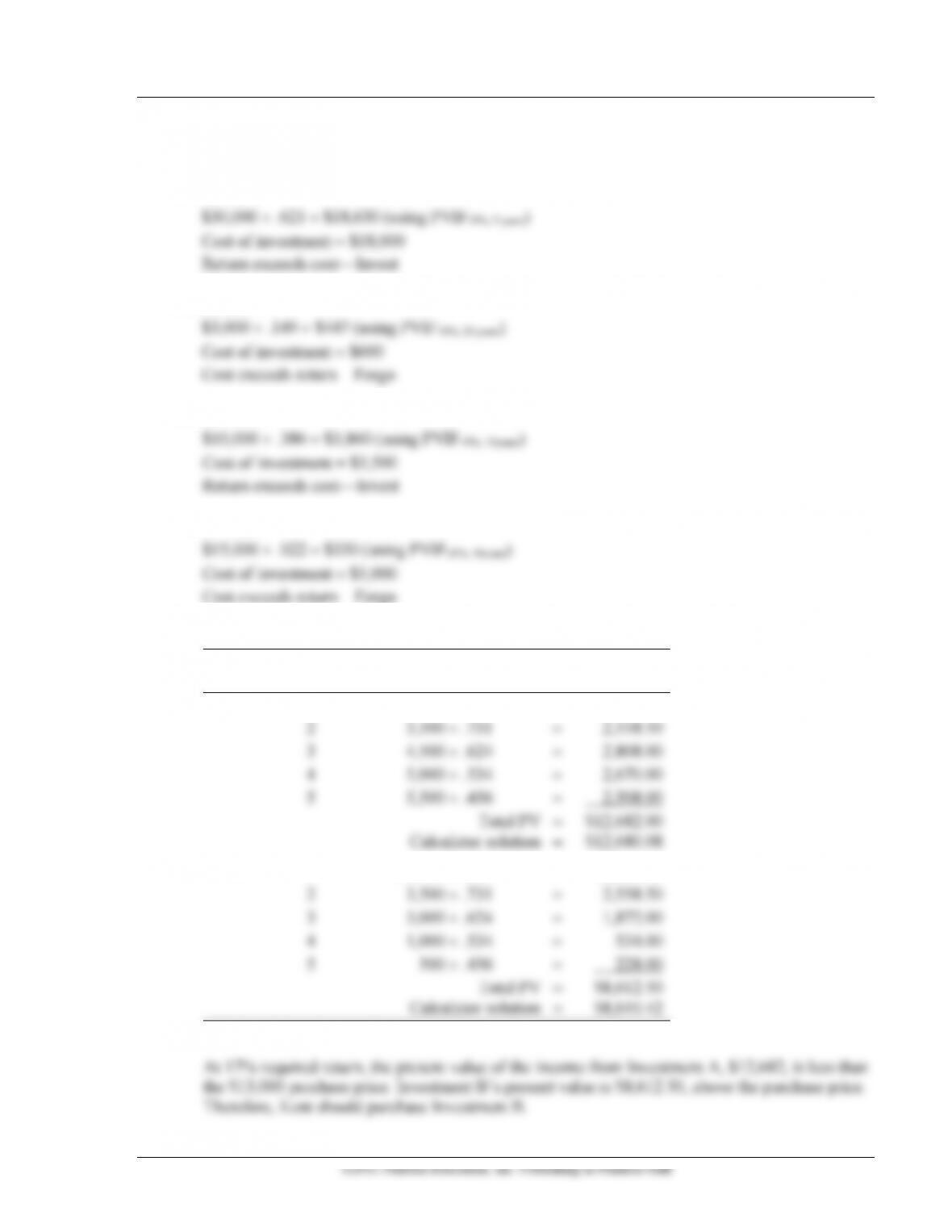
An alternative approach accurately answering the same questions would be the calculation of the
present value of cash inflows and comparing the results to the investment’s cost.
Investment A
Investment B
Investment C
Investment D
4A.18.
Income
Stream
End of
Year
Income PVIF, 17%, n
Present
Value
A
1
$2,500 .855
=
$2,137.50
2
3,500 .731
=
2,558.50
3
4,500 .624
=
2,808.00
4
5,000 .534
=
2,670.00
5
5,500 .456
=
2,508.00
Total PV =
$12,682.00
Calculator solution =
$12,680.08
B
1
$4,000 .855
=
$3,420.00
2
3,500 .731
=
2,558.50
3
3,000 .624
=
1,872.00
4
1,000 .534
=
534.00
5
500 .456
=
228.00
Total PV =
$8,612.50
Calculator solution =
$8,610.42
PVIF from Table A.3, Appendix A.
80 Gitman/Joehnk/Smart • Fundamentals of Investing, Eleventh Edition
4A.19. $15,000 = PVIFA1%, 50 payments PMT
4A.20. Balance is the present value of the payments at 12%. Payments are $382.69. PVIFA1%, 40 periods
◼ Answer to Chapter Opening Problem
The average annual return (% change) in the S&P/Case-Shiller Index is 6.1% (rounding to the nearest