1
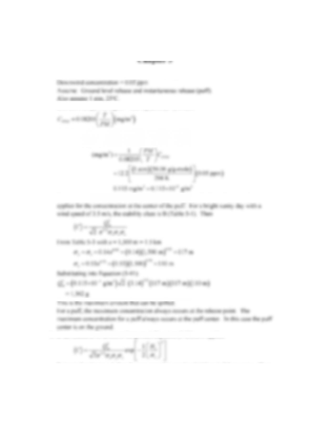
5-1. a. Acrolein C3H4O: M = 56.06 (Appendix E of text)
Convert 0.05 ppm to mg/m3. Use Equation (2-7) in text.
With in K, in atm and in g/g-mole.
T P M
Solve for (mg/m3):
3
3 3 3
1
(mg/m ) 0.08205
1 atm 56.06 g/g-mole
298 K
0.115 mg/m 0.115 10 g/m
PPM
PM C
T
The maximum concentration occurs at the center of the puff. Thus, Equation (5-11)
b. If the release is 10 m above the ground, Equation (5-25) now applies:
2
*
3/ 2
1
2
m r
z
x y z
QH
But note that the term before the exponential is equal to 0.115 mg/m3 from part a. Then:
2
2
3
3
10 m
0.115 mg/m
Note that due to the large value of the z dispersion coefficient, the exponential term has
5-2. a. For this steady state plume, directly downwind on the ground, Equation (5-48) applies:
y z
Q
u
From Table 5-1, for a bright sunny day and 3.5 m/s wind speed, the stability class is B.
With in K, in atm and in g/g-mole.
T P M
Solve for (mg/m3):
3
3 3 3
1
(mg/m ) 0.08205
1 atm 56.06 g/g-mole
298 K
0.115 mg/m 0.115 10 gm/m
PPM
PM C
T
Then, from Table 5-2 at x = 1,500 m for rural conditions and B Stability,
1/2
180 m
Substituting into Equation (5-48):
3 3
0.115 10 g/m 3.14 224 m 180 m 3 m/s
43.7 g/s
m
Q
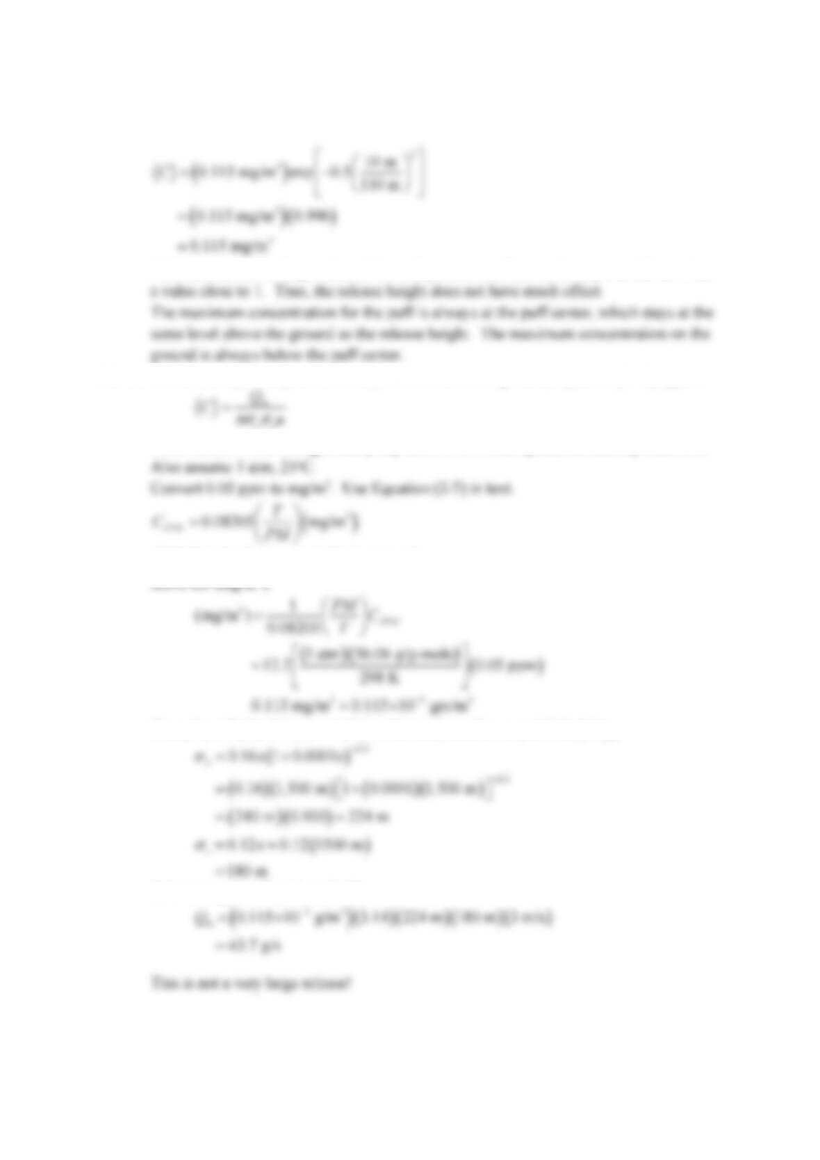
This is not a very large release!
3
b. If the release is 10 m above the ground, Equation (5-20) now applies:
2
1
exp 2
m r
y z z
QH
Cu
But note that the term before the exponential is equal to 0.115 mg/m3 from part a. Then:
2
3
3
10 m
0.1148 mg/m
We can ratio this with the conversion from ppm to mg/m3 from part a:
3
0.05 PPM
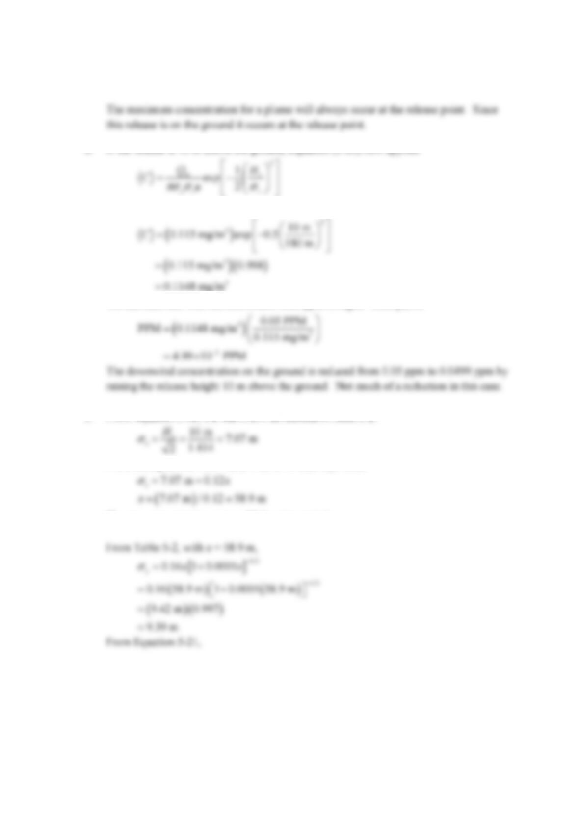
c. From Equation 5-22, the maximum concentration occurs at:
1.414
2
r
z
H
From the equations from Table 5-2, for B-stability, rural,
7.07 m 0.12
zx
The max concentration occurs 58.9 m downwind.
4
2
max
2
2 3
3
2
9.39 m
2.72 3.14 3 m/s 10 m
2.57 10 m/m
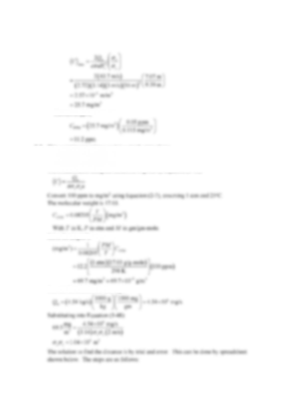
25.7 mg/m
m z
r y
Q
Ce uH
Convert to ppm,
3
0.05 ppm
11.2 ppm
5-3. This a continuous release so it is a steady state plume.
The leak is at ground level.
Assume worst case conditions, F stability and 2 m/s wind speed and rural conditions.
The concentration along the centerline is given by Equation (5-48):
Q
With in K, in atm and in gm/gm–mole.
T P M
Solve for (mg/m3):
3
3 3 3
1
(mg/m ) 0.08205
1 atm 17.03 g/g-mole
298 K
69.7 mg/m 69.7 10 g/m
PPM
PM C
T
Convert the release rate into mg/s
6
1000 g 1000 mg
7.07 m
5
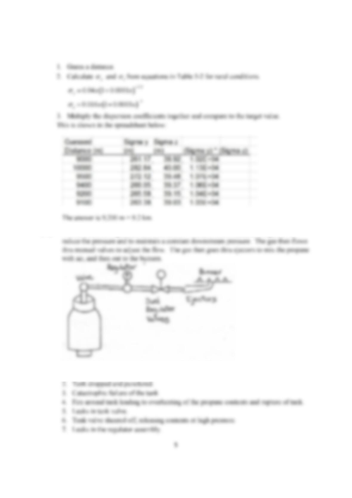
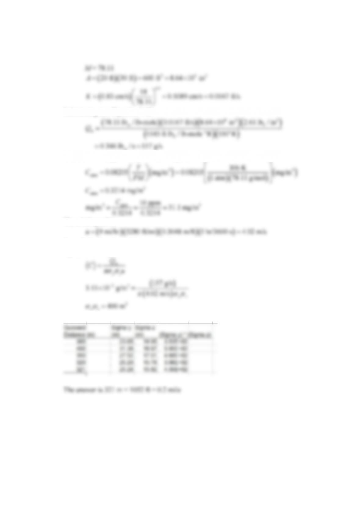
1. Guess a distance.
2. Calculate
y
and
z
from equations in Table 5-2 for rural conditions.
1/2
0.04 1 0.0001
yx x
1
0.016 1 0.0003
z
x x
3. Multiply the dispersion coefficients together and compare to the target value.
This is shown in the spreadsheet below:
The answer is 9,200 m = 9.2 km.
5-4. The hardware configuration is shown below. The tank is connected to a regulator to
Some of the potential release scenarios are:
1. Leaks in the tank
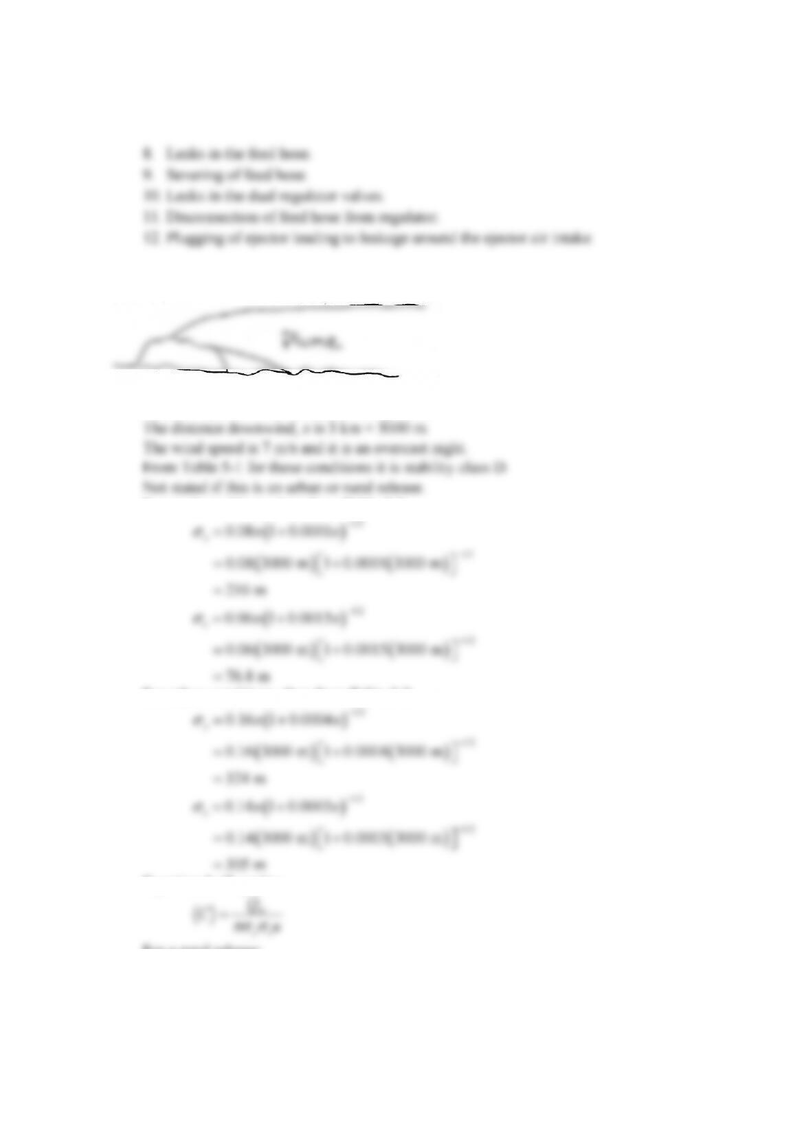
6
Other scenarios are possible.
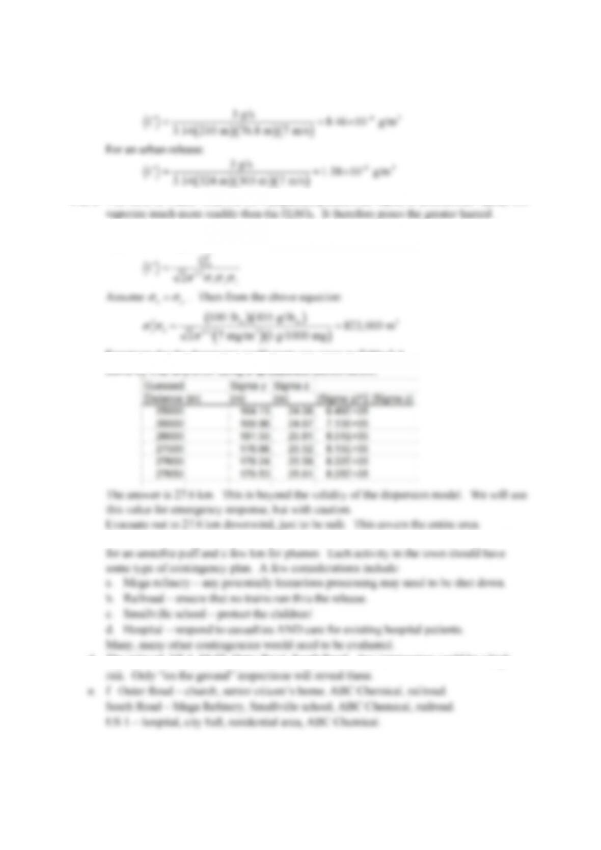
5-5.
This is a burning dump releasing 3 g/s of NOx.
Assume a point source release on the ground.
For rural conditions, then from Table 5-2:
1/2
1/2
1/2
1/2
0.08 1 0.0001
0.08 3000 m 1 0.0001 3000 m
210 m
0.06 1 0.0015
0.06 3000 m 1 0.0015 3000 m
76.8 m
y
z
x x
x x
For urban conditions, then from Table 5-2:
1/2
1/2
1/2
1/2
0.16 1 0.0004
0.16 3000 m 1 0.0004 3000 m
324 m
0.14 1 0.0003
0.14 3000 m 1 0.0003 3000 m
305 m
y
z
x x
x x
Equation 5-17 applies:
y z
Q
u
For a rural release:
7
6 3
3 g/s
8.46 10 g/m
C
3.14 324 m 305 m 7 m/s
5-6. a. The HCl, no matter what the form (aqueous, pressurized vapor, or pressurized liquid, will
b. Assume worst case: a puff, stable conditions.
Equation 5-11 applies:
*
m
Q
3/2 3
2 7 mg/m 1 g/1000 mg
y z
Equations for the dispersion coefficients are given in Table 5-3.
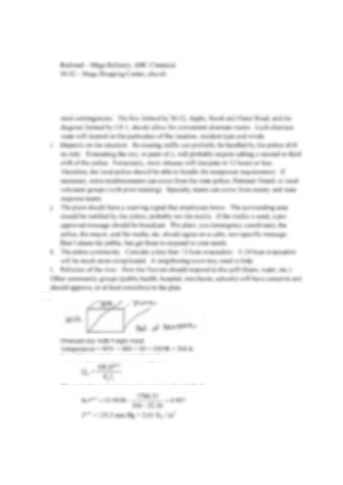
Solve by trial and error using a spreadsheet shown below:
c. The entire town may be affected by the release. A typical evacuation area is about 1 km
d. The railroad, US 1, M-52, Outer Road, South Road. Any intersection could be a high
6 3
1.38 10 g/m
8
g. Generally, evacuate toward the NE, away from the prevailing winds. However, this will
vary from day to day. Consider using the Smallville School, if the winds allow. Several
evacuation sites should be pre-planned and pre-coordinated.
h. The police should have experience doing this. Ensure that their plans adequately cover
5-7.
From Chapter 3, Equation 3-12 applies:
sat
m
g L
MKAP
QR T
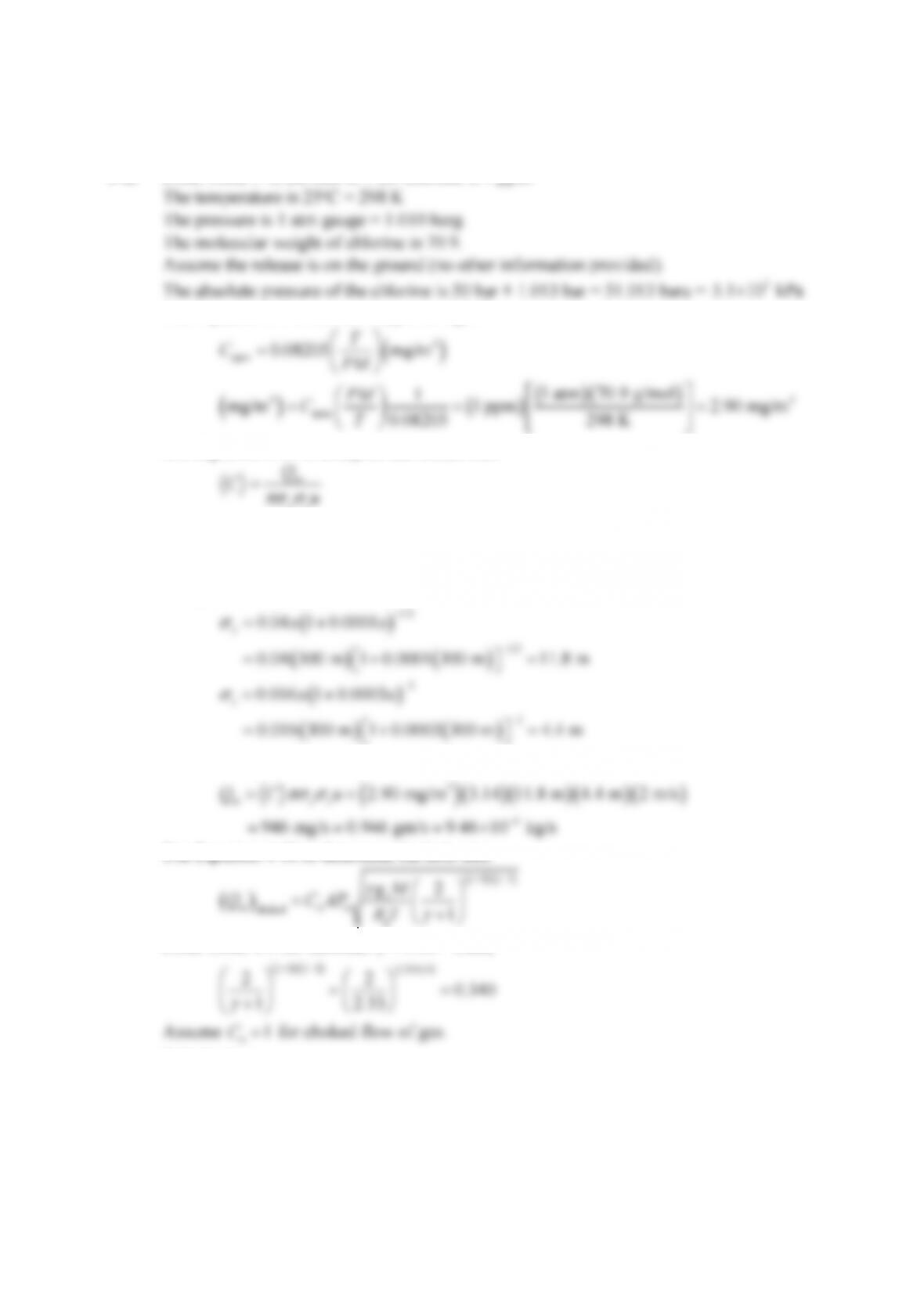
The saturation vapor pressure is given in Appendix C:
2
f
2788.51
ln 15.9008 4.907
306 52.36
135.2 mm Hg = 2.61 lb / in
sat
sat
P
P
9
Substituting into Equation 3-12:
4 2 2
m f
o o
f
m
78.11 lb / lb–mole 0.0167 ft/s 8.64 10 in 2.61
lb / in
0.346 lb / s 157 g/s
m
Q
Need to convert ppm to mg/m3. Use Equation 2-7:
3 3
ppm
3
ppm
ppm
3 3
306 K
0.08205 mg/m 0.08205 mg/m
1 atm 78.11 g/mol
10 ppm
mg/m 31.1 mg/m
0.3214 0.3214
T
CPM
C
The wind speed is:
9 mi/hr 5280 ft/mi 0.3048 m/ft 1 hr/3600 s 4
.02 m/s
u
From Table 5-1, the stability class is D.
Equation 5-17 applies:
m
2
400 m
y z
y z
y z
Q
Cu
Solve by trial and error using a spreadsheet:
20 ft 30 ft 600 ft 8.64 10 in
10
5-8. From Table 5-4, the ERPG-1 for chlorine is 1 ppm.
Use Equation 2-7 to convert 1 ppm to mg/m3:
3
ppm
3 3
ppm
0.08205 mg/m
1 atm 70.9 g/mol
1
mg/m 1 ppm 2.90 mg/m
0.08205 298 K
T
CPM
PM
CT
Use Equation 5-17 to compute the release rate:
y z
Q
u
Without any additional information, assume worst case conditions, i.e. F-stability and
2 m/s windspeed and rural conditions.
Then, from Table 5-2:
0.04 300 m 1 0.0001 300 m 11.8 m
1/2
1
1
0.016 1 0.0003
0.016 300 m 1 0.0003 300 m 4.4 m
z
x x
Solve for
m
Q
:
3
2.90 mg/m 3.14 11.8 m 4.4 m 2 m/s
m y z
Q C u
Use Equation 4-50 to determine the hole size:
1 / 1
c
2
g M
From Table 4-3 for chlorine,
1.33
. Then,
1 / 1 2.33/0.33
2 2
Substituting:
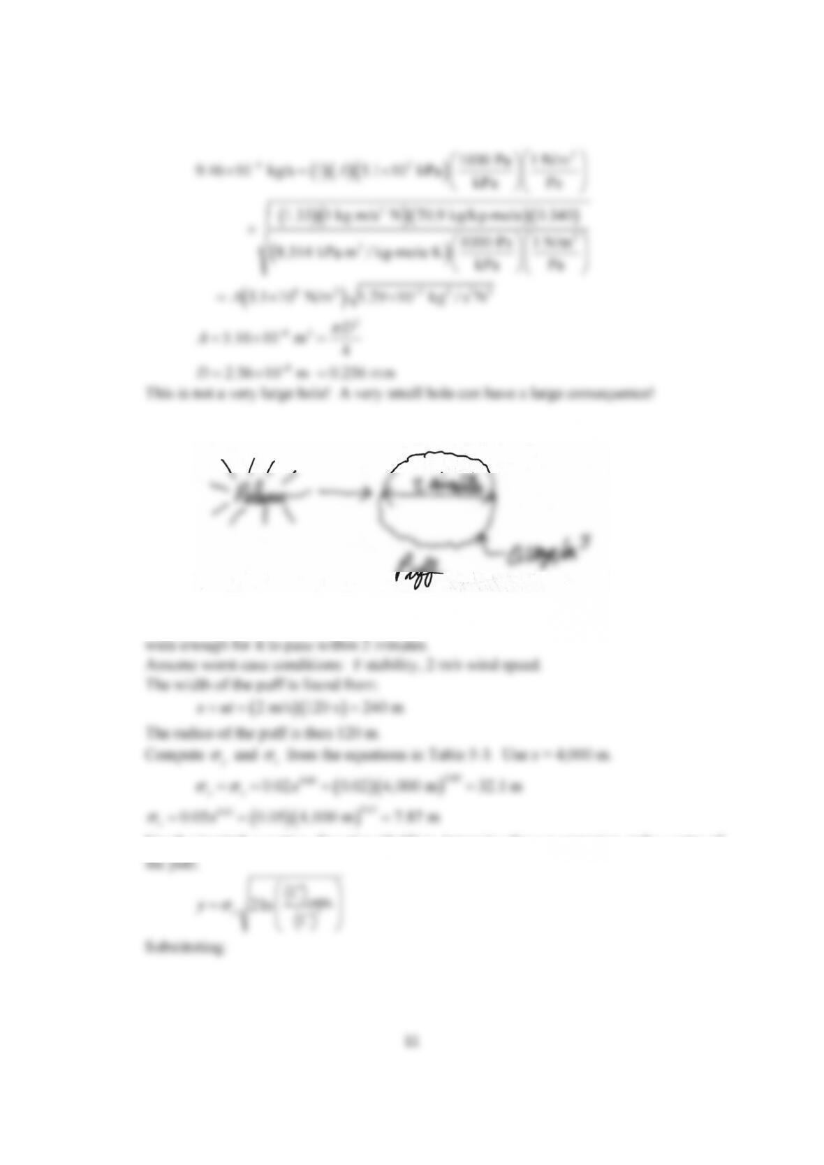
11
2
4 3
2
2
3
6 2 5 2 2 2
1000 Pa 1 N/m
9.46 10 kg/s 1 5.1 10 kPa kPa Pa
1.33 1 kg m/s N 70.9 kg/kg-mole 0.340
1000 Pa 1 N/m
8.314 kPa m / kg-mole K kPa Pa
5.1 10 N/m 1.29 10 kg / s N
A
A
2
8 2
8
5.16 10 m 4
2.56 10 m 0.256 mm
D
A
D
This is not a very large hole! A very small hole can have a large consequence!
5-9.
To solve this problem, we need to determine the instantaneous release which results in a
puff 4,000 m downwind with an isopleth of 0.1 mg/m3. The width of the puff must be
zx
Use the isopleth equation, Equation (5-45) to determine the concentration at the center of
2 m/s 120 s 240 m
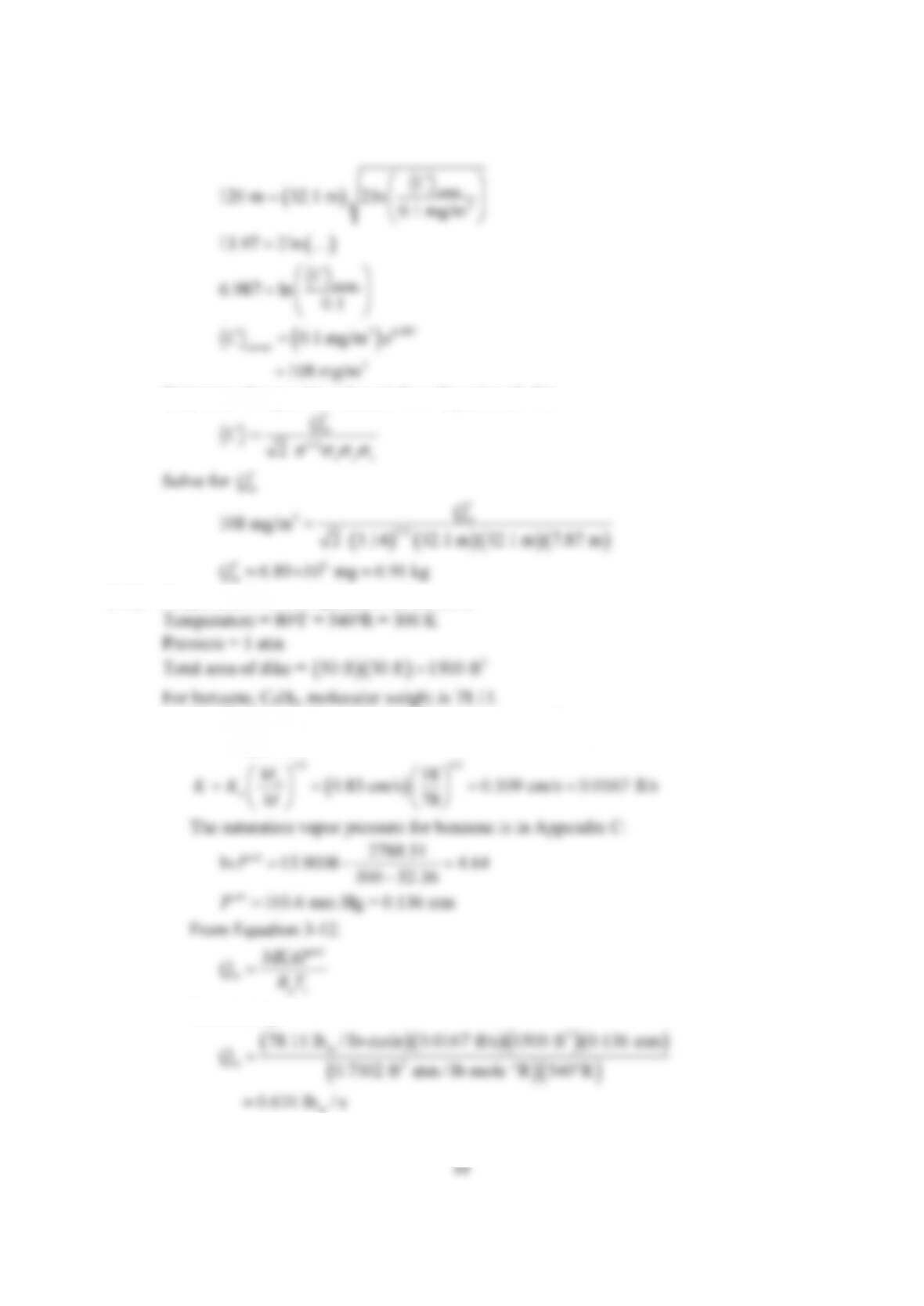
center
3
center
3 6.987
center
3
120 m 32.1 m 2ln
0.1 mg/m
13.97 2ln ….
0.1 mg/m
108 mg/m
C
C
C e
Determine the quantity released from Equation (5-41):
*
m
Q
* 6
6.89 10 mg 6.91 kg
m
Q
5-10. Evaporation from a liquid pool of benzene.
a. Use Equation 3-12 and 3-18 to determine evaporation rate.
From Equation 3-18:
1/3 1/3
18
o
M
m
g L
Substituting,
2
m
3 o o
m
78.11 lb / lb-mole 0.0167 ft/s 1500 ft 0.136
atm
0.674 lb / s
m
Q
b. From Appendix E for benzene:
13
y z
u
Substituting:
3.14 2.23 m/s
5
3
2
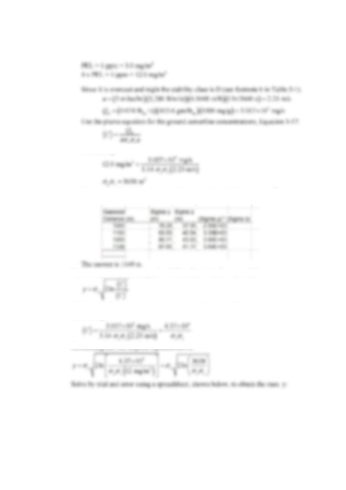
3.057 10 mg/s
12.0 mg/m
3638 m
y z
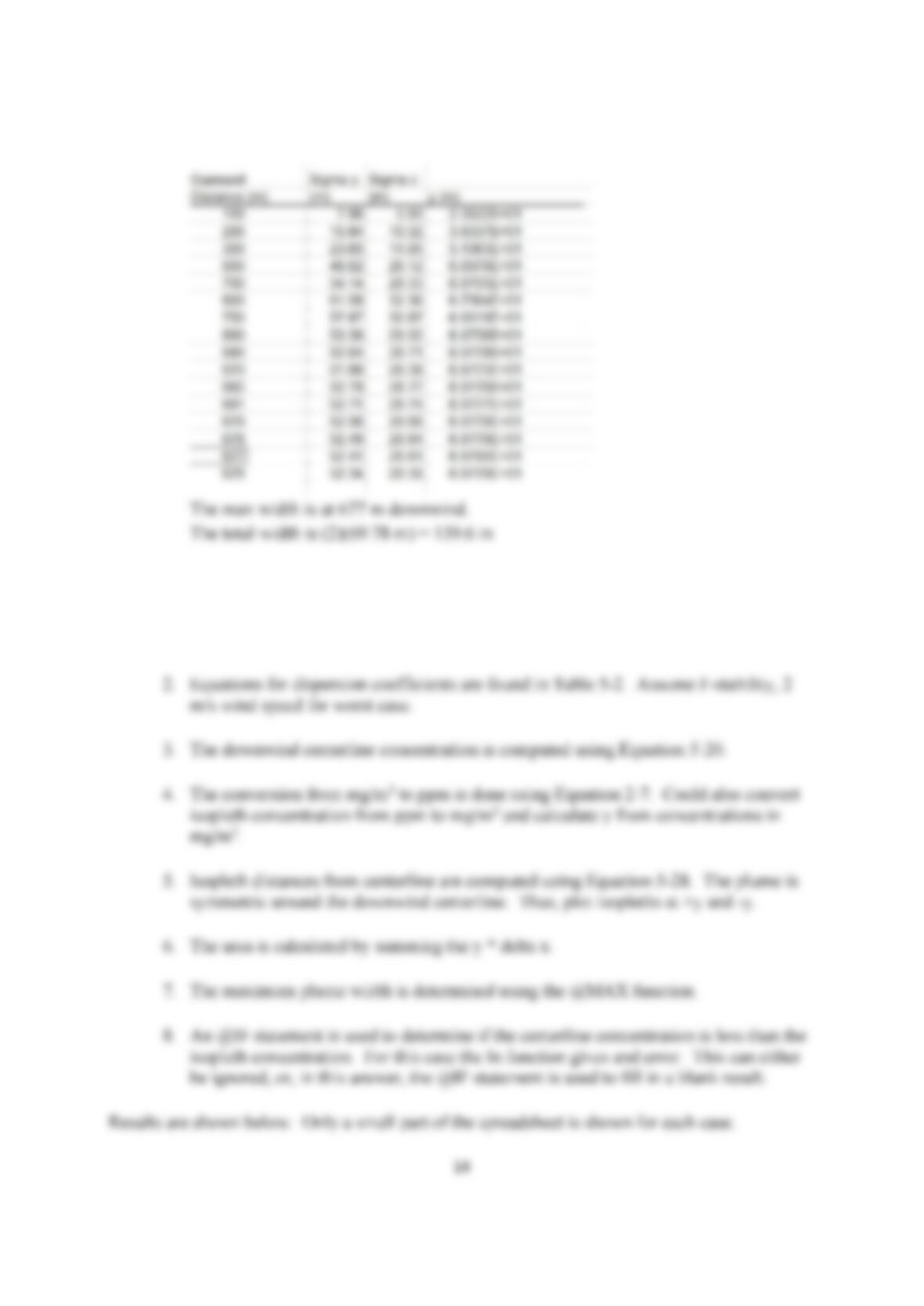
This is solved by trial and error solution using the rural dispersion coefficients
equations in Table 5-2. The spreadsheet solution is shown below:
c. Use the isopleth equation, equation 5-28 to determine the max. width.
*
y
C
C
But the centerline concentration is found using Equation 5-17 shown above.
Substituting,
5 4
3.057 10 mg/s 4.37 10
3.14 2.23 m/s
y z y z
Substituting into the isopleth equation above:
4
3
4.37 10 3638
2ln 2ln
y y
y
14
The max width is at 677 m downwind.
The total width is (2)(69.78 m) = 139.6 m
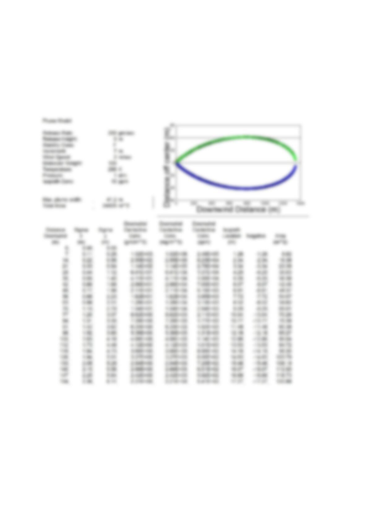
5-11. Use the following considerations to develop your spreadsheet:
1. Break up the plume into fixed spatial increments, say 7 m. The result is not
dependent on this selection – it only affects the plot precision.
15
The plume length and width on the ground is significantly decreased as the release height
increases.
Part a:
5-12. The most direct approach is to use a coordinate system that is fixed on the ground at the
release point. Thus, Equation 5-25 is used with Equation 5-27. This gives,
2
2
*
3/2
1 1
2 2
2
m r
z x
x y z
Q H x ut
Note that ut is the location of the center of the puff.
In order to reduce the number of spreadsheet cells, use a spreadsheet grid that moves with
the puff center. Use, let’s say, 50 cells on either side of the puff and specify a cell
increment size.
The procedure is the following: