Supplement
I
Learning Curve Analysis
PROBLEMS
Developing Learning Curves
1. Mass Balance Company
a.
Time for the second unit
Time for the first unit
48
60
0.8
r=
=
=
b.
( )
( )
1
40
0.321928
log log 2
log 0.80 log 2
0.321928
60 40
18.30 hr
b
n
br
k k n
k−
=
=
=−
=
=
=
c. Estimated total time for 40 units, from Table I.1, conversion factor = 0.42984.
d. Estimated total time for 30 units, from Table I.1, conversion factor = 0.46733.
⚫
SUPPLEMENT I
⚫
Learning Curve Analysis
I-2
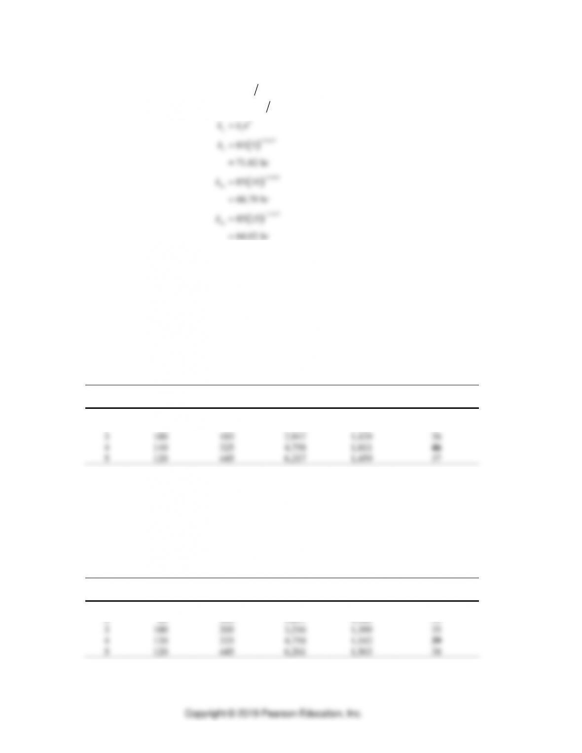
2. Cambridge Instruments
( )
( )
( )
1
0.1047
5
0.1047
10
0.1047
15
0.1047
30
log log 2
log 0.93 log 2 0.1047
85 5
71.82 hr
66.79 hr
85 15
64.02 hr
85 30
59.53 hr
b
n
br
k k n
k
k
k
−
−
−
−
=
= = −
=
=
=
=
=
=
=
=
Using Learning Curves
3. A large grocery corporation
The first unit required 30 hours.
130k=
. We can use Table I.1 and straight-line
interpolation to get the cumulative average time factor for a 90 percent learning
curve. The following solution was developed with the use of a computer routine.
Units
Cumulative
Cumulative
Total
Total
Week
Scheduled
Production
Total Hr
Hr/Wk
Employees/Wk
1
20
20
438
438
11
2
65
85
1,518
1,080
27
3
100
185
2,947
1,429
36
4
140
325
4,758
1,811
46
5
120
445
6,217
1,459
37
The production schedule is not feasible because the number of employees needed in
week 4 exceeds the maximum of 40 by 6 workers.
To obtain a feasible schedule, we can produce some of the requirements in week 4
earlier, say in week 2 or 3. Such a change may result in excess inventory cost if the
customer does not accept early shipment. Furthermore, the production schedule of
other products may be affected by this alternative.
One possible production schedule is:
Units
Cumulative
Cumulative
Total
Total
Week
Scheduled
Production
Total Hr
Hr/Wk
Employees/Wk
1
20
20
438
438
11
2
85
105
1,817
1,381
35
3
100
205
3,216
1,399
35
4
120
325
4,758
1,542
39
5
120
445
6,261
1,503
38
Learning Curve Analysis
⚫
SUPPLEMENT I
⚫
I-3
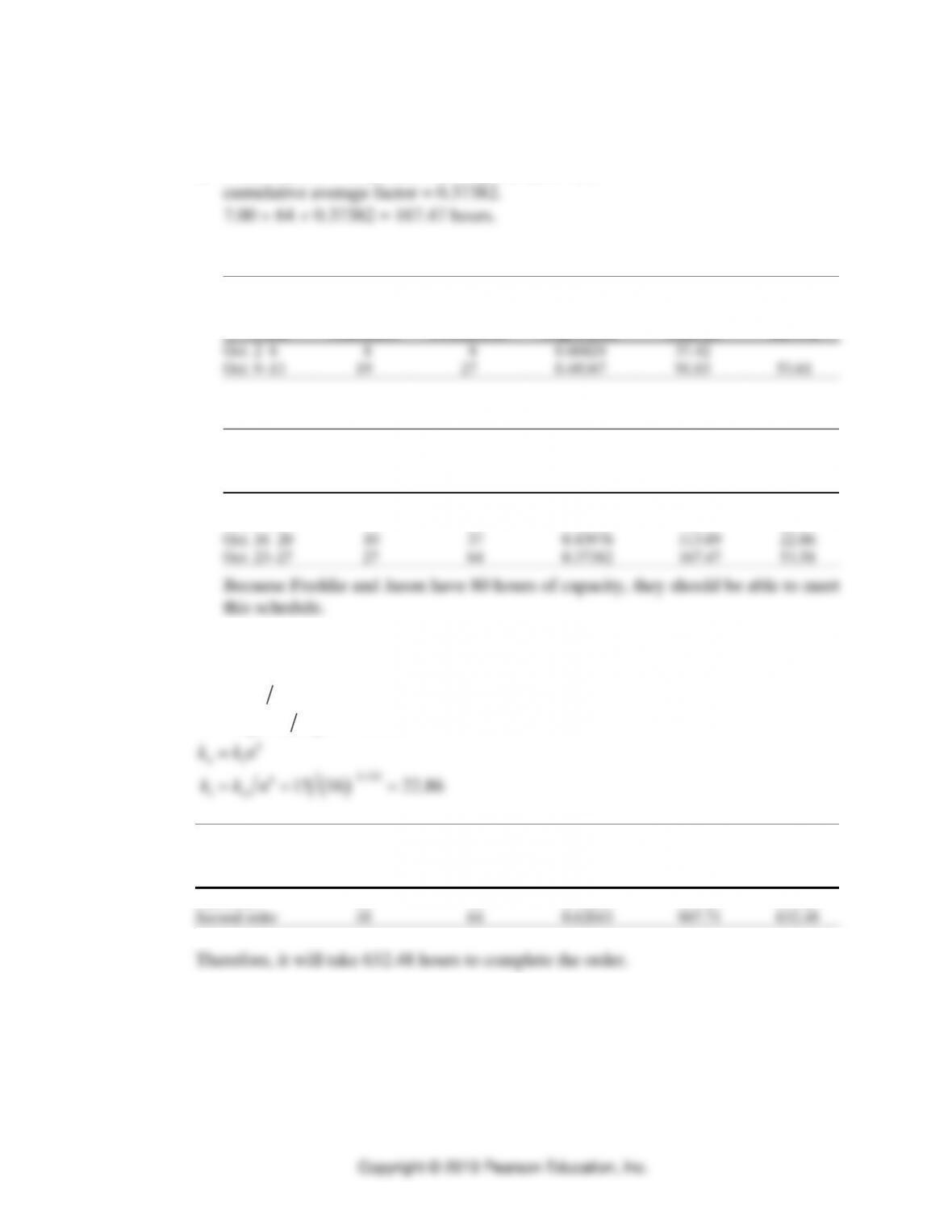
4. Texas Toothpick.
17.00k=
a. From Table I.1, 80 percent learning curve, n = 64,
b. Week of Friday the 13th
(1)
(2)
1
k
(1) (2)
Units
Cumulative
Cumulative
Cumulative
Total
Week
Scheduled
Production
Avg. Factor
Total Hr
Hr/Wk
Oct. 2–6
8
8
0.66824
37.42
Oct. 9–13
19
27
0.48167
91.03
53.61
c. Week before Halloween
(1)
(2)
1
k
(1) (2)
Units
Cumulative
Cumulative
Cumulative
Total
Week
Scheduled
Production
Avg. Factor
Total Hr
Hr/Wk
Oct. 2–6
8
8
0.66824
37.42
Oct. 9–13
19
27
0.48167
91.03
53.61
Oct. 16–20
10
37
0.43976
113.89
22.86
Oct. 23–27
27
64
0.37382
167.47
53.58
5. Bovine Products Company. We know the time required for the 16th unit. We need to
use a 90% learning curve and work backwards to estimate the time for the 1st unit.
(1)
(2)
(1) (2)
Cumulative
Cumulative
Cumulative
Hours/
Scheduled
Production
Avg. Factor
Total Hr
Order
First order
16
16
0.75249
275.23
Second order
48
64
0.62043
907.71
log log2
log0.90 log2 0.152
br
b
=
= = −
⚫
SUPPLEMENT I
⚫
Learning Curve Analysis
I-4
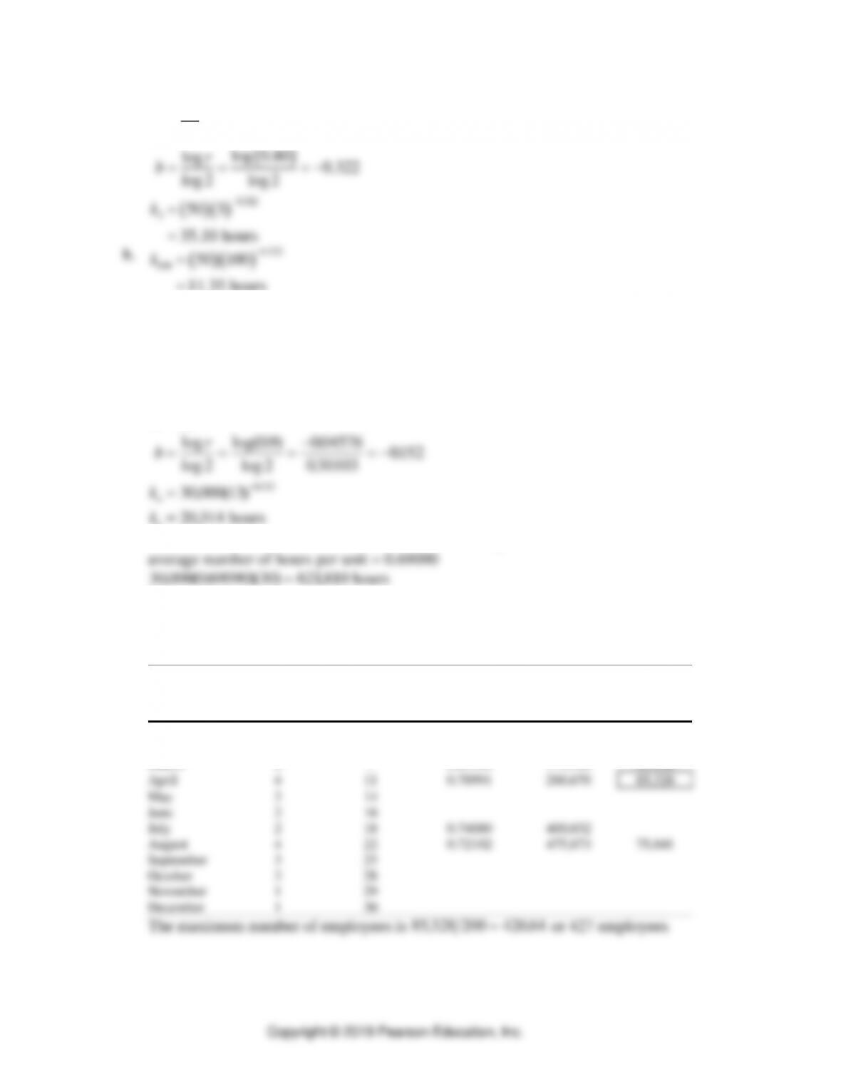
a.
( )
( )( )
0.322
3
40 0.80
50
log 0.80
log 0.322
log2 log2
50 3
35.10 hours
r
r
b
k−
==
= = = −
=
=
b.
( )( )
0.322
100 50 100
11.35 hours
k−
=
=
c. Average time per unit over a total order of 1000 units (using factor from Table I.1
for r = 80% and n = 1,000, (50)(0.15867) = 7.93 hours. The contract’s assumption
is valid.
7. Powerwest Inc.
a. Direct hours for the thirtieth unit
k k n
br
k
k
nb
n
n
=
= = ( ) =−= −
=( )
=
−
1
0152
09
004576
30 000 13
20 314
log
log .
.
,
,
.
hours
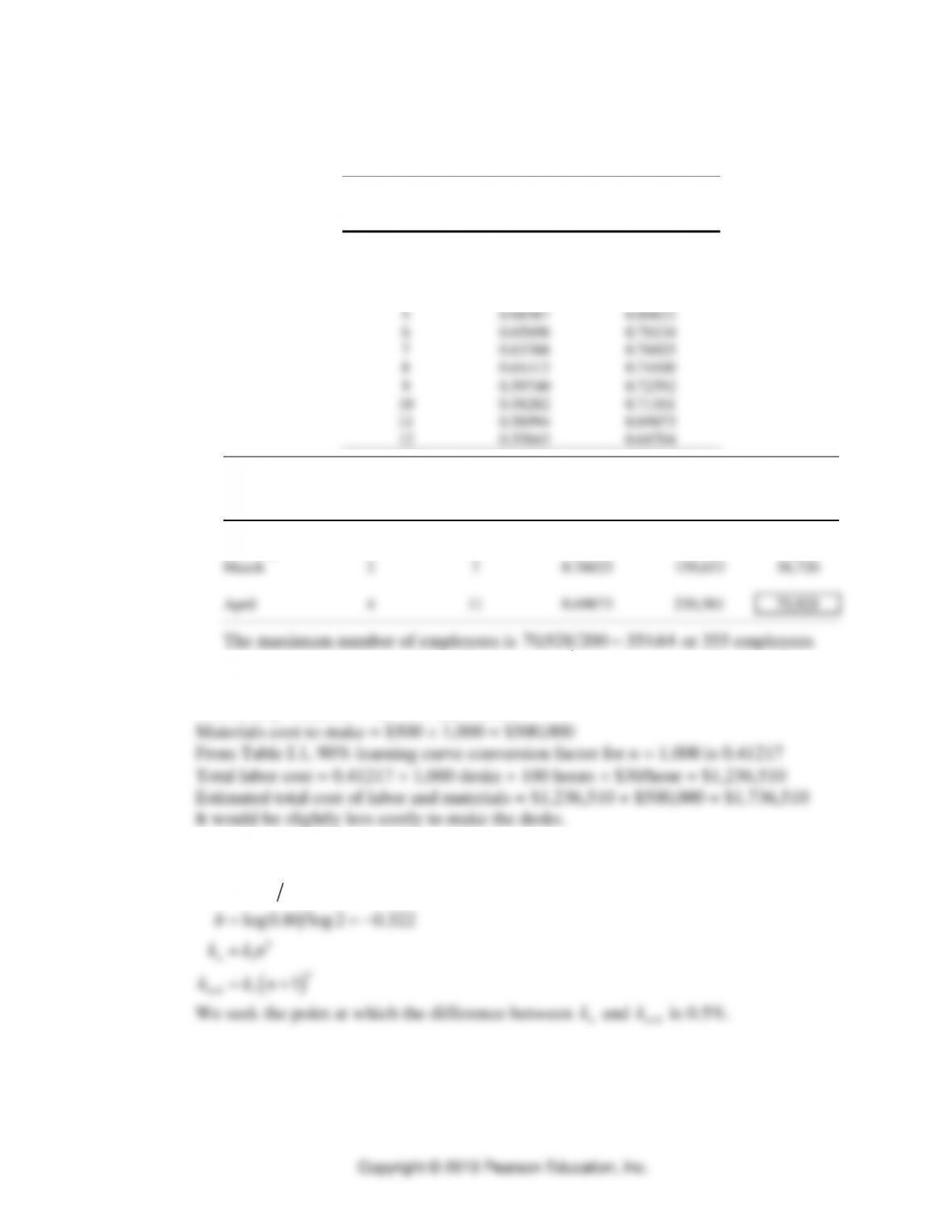
b. Total hours for 30 units. From Table I.1 90% learning curve, conversion factor for
c. By inspection the maximum number of employees will occur sometime during the
first four months. Because of the learning effect, production following April
cannot possibly exceed the hours required for April. For example, the four units in
August require about 9,500 fewer hours than do the four units in April.
Month
Units
Scheduled
(1)
Cumulative
Production
(2)
Cumulative
Avg. Factor
1
k
(1) (2)
Cumulative
Total Hr
Hours/
Month
January
2
2
0.95000
57,000
57,000
February
3
5
0.86784
130,176
73,176
March
2
7
0.83496
175,342
45,166
April
4
11
0.78991
260,670
85,328
May
3
14
June
2
16
July
2
18
0.74080
400,032
August
4
22
0.72102
475,873
75,841
September
3
25
October
3
28
November
1
29
December
1
30
The maximum number of employees is
85328 200 42664, .=
or 427 employees
Learning Curve Analysis
⚫
SUPPLEMENT I
⚫
I-5
d. If the learning curve is changed to 0.85, we cannot use Table I.1 to find the
cumulative average factor. We have used a spreadsheet to generate the cumulative
average factor for a learning rate of 85%.
Learning Rate
85%
b =
–0.2344653
Cumutative
N
kn
Average Factor
1
1.00000
1.00000
2
0.85000
0.92500
3
0.77291
0.87430
4
0.72250
0.89635
5
0.68567
0.80622
6
0.65698
0.78134
7
0.63388
0.76025
8
0.61413
0.74100
9
0.59740
0.72592
10
0.58282
0.71161
11
0.58994
0.69873
12
0.55843
0.68704
Month
Units
Scheduled
(1)
Cumulative
Production
(2)
Cumulative
Avg. Factor
1
k
(1) (2)
Cumulative
Total Hr
Hours/
Month
January
2
2
0.92500
55,500
55,500
February
3
5
0.80622
120,933
65,433
March
2
7
0.76025
159,653
38,720
April
4
11
0.69873
230,581
70,928
The maximum number of employees is
70 928 200 35464, .=
or 355 employees
8. Really Big Six Corporation
Cost to buy = $2,000
1,000 = $2,000,000
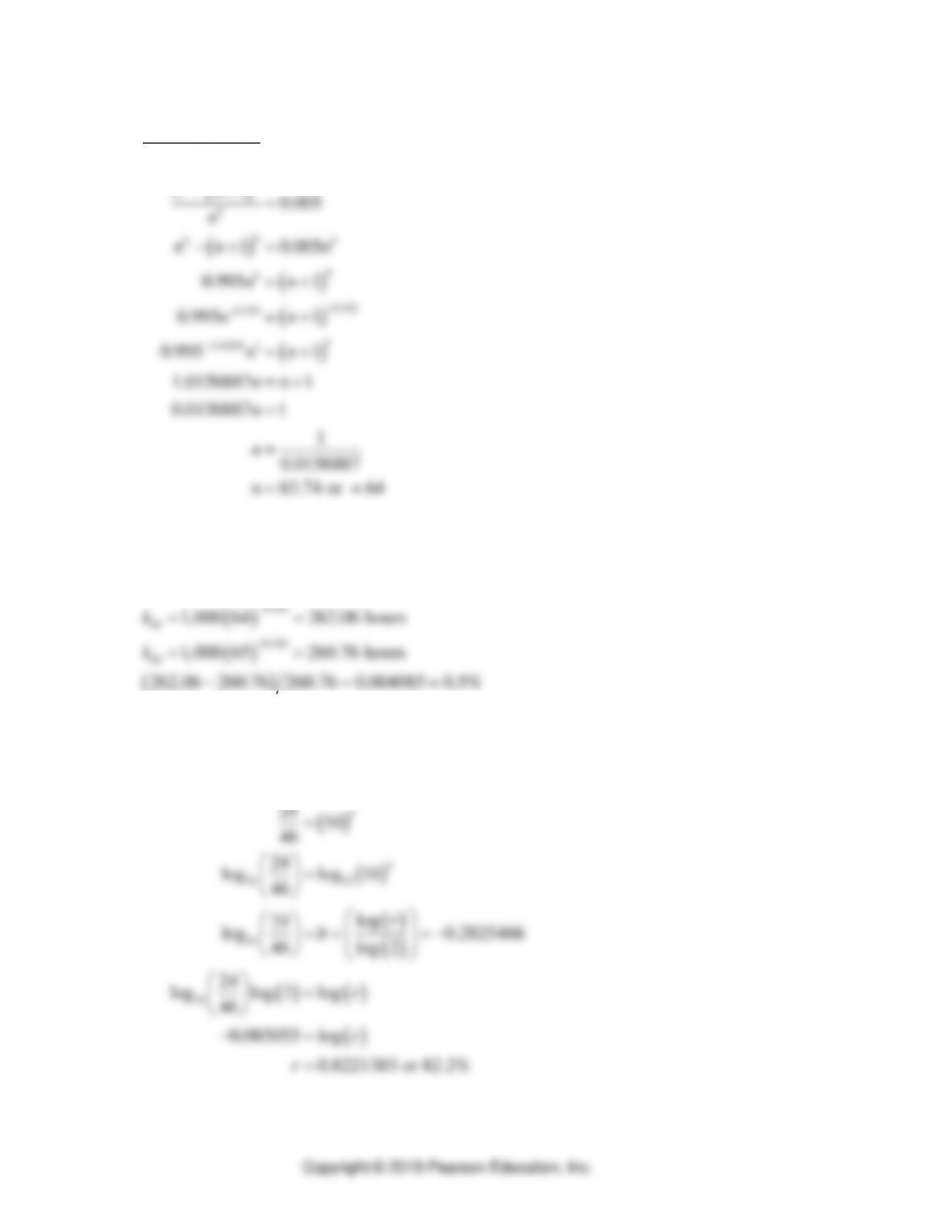
9. When the learning curve is 80%
log log2
log0.80 log2 0.322
br
b
=
= = −
⚫
SUPPLEMENT I
⚫
Learning Curve Analysis
I-6
( )
( )
( )
( )
( )
( )
11
1
0.322
0.322
1
3.10559 1
10.005
10.005
1 0.005
0.995 1
0.995 1
0.995 1
1.0156887 1
0.0156887 1
1
0.0156887
63.74 or 64
b
b
b
b
b
b
b
bb
b
b
k n k n
kn
nn
n
n n n
nn
nn
nn
nn
n
n
n
−
−
−
−+
=
−+ =
− + =
=+
=+
=+
=+
=
=
=
Check:
Say
1,000
l
k=
hours, n = 64, and learning curve is 80%.
1
0.322
b
n
k k n
−
=
Learning Curve Analysis
⚫
SUPPLEMENT I
⚫
I-7
b. Given
46
l
k=
hours and the estimated learning curve rate from part a,
( )( )
( )
0.28252466
80
80
46 80
13.338 hours
k
k
−
=
=
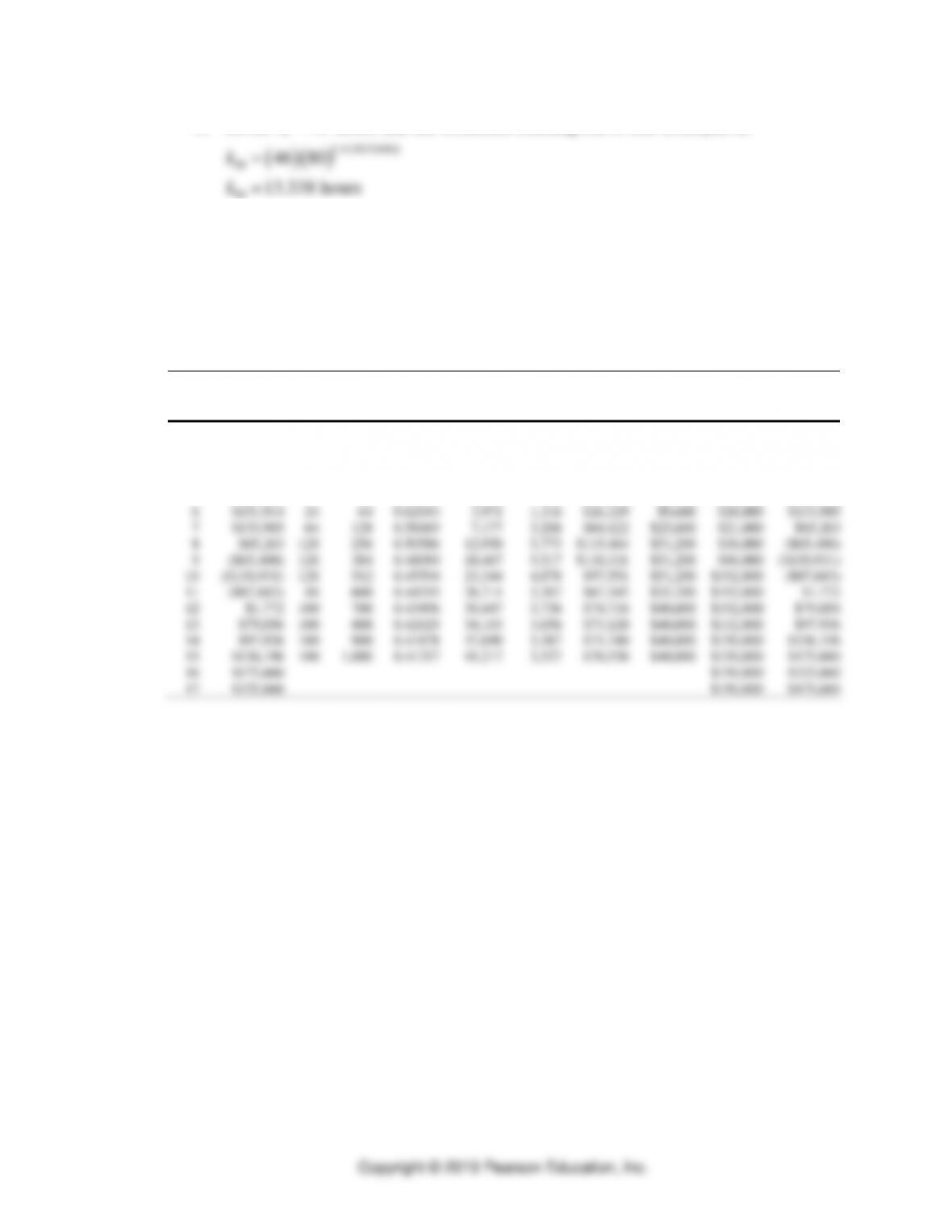
11. Hand-To-Mouth Company
Poor cash management is the number one cause of bankruptcy. The following
spreadsheet shows the calculation of cash flow. HTM must not take this order unless
they are assured they can obtain a loan to cover the cash shortages occurring in weeks
8–10. Some of the values for the cumulative average hours factor were interpolated
from data in Table I.1. Tabular values below may have slight rounding-off errors.
Cum.
Cum. Avg.
Cum.
Ending
Beginning
Del.
Contr.
Hours
Labor
Labor
Labor
Material
Cash
Cash
Week
Cash
Units
Units
Table I.1
Hours
Hours
Costs
Costs
Received
Balance
1
$200,000
2
2
0.95000
190
190
$3,800
$800
$195,400
2
$195,400
4
6
0.85013
510
320
$6,402
$1,600
$187,398
3
$187,398
8
14
0.76580
1,072
562
$11,241
$3,200
$3,000
$175,958
4
$175,958
12
26
0.70472
1,832
760
$15,203
$4,800
$6,000
$161,955
5
$161,955
14
40
0.66357
2,654
822
$16,440
$5,600
$12,000
$151,914
6
$151,914
24
64
0.62043
3,971
1,316
$26,329
$9,600
$18,000
$133,985
7
$133,985
64
128
0.56069
7,177
3,206
$64,122
$25,600
$21,000
$65,263
8
$65,263
128
256
0.50586
12,950
5,773
$115,464
$51,200
$36,000
($65,400)
9
($65,400)
128
384
0.48090
18,467
5,517
$110,331
$51,200
$96,000
($130,931)
10
($130,931)
128
512
0.45594
23,344
4,878
$97,551
$51,200
$192,000
($87,683)
11
($87,683)
88
600
0.44519
26,711
3,367
$67,345
$35,200
$192,000
$1,772
12
$1,772
100
700
0.43496
30,447
3,736
$74,716
$40,000
$192,000
$79,056
13
$79,056
100
800
0.42629
34,103
3,656
$73,120
$40,000
$132,000
$97,936
14
$97,936
100
900
0.41878
37,690
3,587
$71,740
$40,000
$150,000
$136,196
15
$136,196
100
1,000
0.41217
41,217
3,527
$70,536
$40,000
$150,000
$175,660
16
$175,660
$150,000
$325,660
17
$325,660
$150,000
$475,660