Supplement
H
Measuring Output Rates
PROBLEMS
Time Study Method
1. A machine shop
a. Normal time per cycle = (Average observed time)(Rating factor)
The average observed time is: (40 + 48 + 48 + 46 + 42)/5 = 44.80 min./operation
The normal time per cycle is then:
b. Standard time = Normal time for the cycle (1.0 + allowance):
( )
1.0
48.94 min.
ST NTC A=+
=
2 Stetson and Stetson Company
a. Normal time per cycle = (Average observed time)(Rating factor)
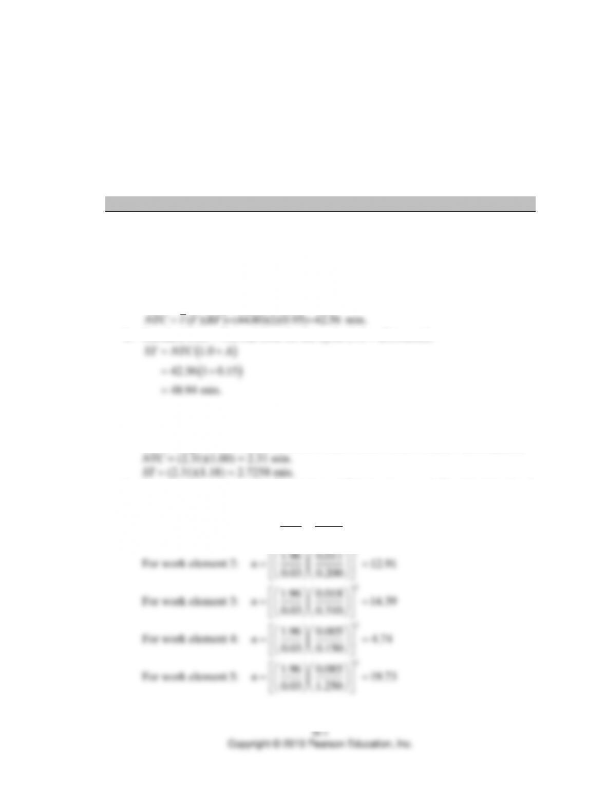
The average observed time is: (0.40 + 0.20 + 0.31 + 0.15 + 1.25) = 2.31 minutes
b. Sample size necessary for 95 percent confidence, i.e., z = 1.96 and error of 3
percent:
For work element 1:
2
1.96 0.021 11.76
0.03 0.400
==
n
2
1.96 0.011 12.91
0.03 0.200
For work element 3:
2
1.96 0.018 14.39
0.03 0.310
==
n
For work element 4:
2
1.96 0.005 4.74
0.03 0.150
==
n
For work element 5:
2
1.96 0.085 19.73
0.03 1.250
==
n
⚫
SUPPLEMENT H Measuring Output Rates
⚫
H-2
c. Sample size of 20 is adequate.
3. Bill’s Fast-Food Restaurant
Work
Element
1
2
3
4
5
t
RF
F
NT
1
0.45
0.41
0.50
0.48
0.36
0.44
0.9
1
0.396
2
0.85
0.81
0.77
0.89
0.83
0.83
1.2
1
0.996
3
0.60
0.55
0.59
0.58
0.63
0.59
1.2
1
0.708
4
0.31
0.24
0.27
0.26
0.32
0.28
1.0
1
0.280
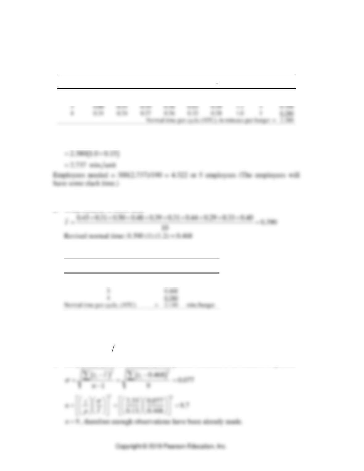
Normal time per cycle (NTC), in minutes per burger
=
2.380
Standard time = Normal time per cycle (1.0 + allowance)
( )
1.0
2.737 min. unit
ST NTC A=+
=
Employees needed = 300(2.737)/190 = 4.322 or 5 employees (The employees will
have some slack time.)
4. Bill’s Fast-Food Restaurant, continued
a. Work element 3, select time
0.45 0.31 0.50 0.48 0.39 0.31 0.44 0.29 0.33 0.40 0.390
+ + + + + + + + +
b. Revised normal time per cycle.
Work
Element
NT
1
0.396
2
0.996
3
0.468
4
0.280
Normal time per cycle, (NTC)
=
2.140
min./burger
Revised standard time per cycle
( )
( )
1.0
2.140 1.0 0.15
2.461 min. burger
ST NTC A=+
=+
=
c. Sample size for work element 3,—98 percent confident to be within
13 percent
( ) ( )
22
0.468 0.077
−−
ii
t t t
Measuring Output Rates
⚫
SUPPLEMENT H
⚫
H-3
d. Number of employees required when 3rd work element is inflated by 13%.
Standard time (3rd work element time is increased by 13%).
There is often little or no trust between management and labor. In such an
environment, the suspicious cook will not tell management about his improved
method. He would be concerned that a coworker would be fired and those
remaining would have to work harder.
5. Black Sheep Wool Company
The following table contains the data needed to compute the normal time per cycle.
Work
Element
1
2
3
4
5
6
7
8
9
10
11
12
t
F
RF
NT
1 fill
0.20
0.22
0.24
0.18
0.20
0.21
0.22
0.19
0.24
0.18
0.19
0.25
0.21
1.00
1.2
0.252
2 sew
0.40
0.38
0.37
0.41
0.41
0.40
0.36
0.37
0.41
0.42
0.39
0.36
0.39
1.00
0.8
0.312
3 transport
—
—
0.82
—
—
0.84
—
—
0.73
—
—
0.85
0.81
0.33
1.1
0.294
6. Super-Fast Speedway
The following table shows the elapsed times for each of the observations, the average
time and normal time for each work element, and the normal time for the (left plus
right side) cycle. The time between pit stops is not relevant to the study.
Observed cycle number
1
2
3
4
5
6
Work
Left
Right
Left
Right
Left
Right
Element
side
side
side
side
side
side
t
F
RF
NT
1. Wait for car lift
2.9
—
3.2
—
2.6
—
2.9
0.5
1.0
1.45
2. Remove lugs
3.3
3.8
3.6
3.8
4.0
4.3
3.8
1
0.9
3.42
3. Switch tires
6.4
7.1
6.8
7.3
6.2
6.4
6.7
1
1.2
8.04
4. Tighten lugs
4.1
3.8
3.5
4.9
3.5
4.2
4.0
1
0.8
3.20
5. Move to right side
3.8
—
4.3
—
3.2
—
3.77
0.5
1.2
2.26
6. Clear away for drop
—
2.1
—
2.7
—
2.0
2.27
0.5
0.9
1.02
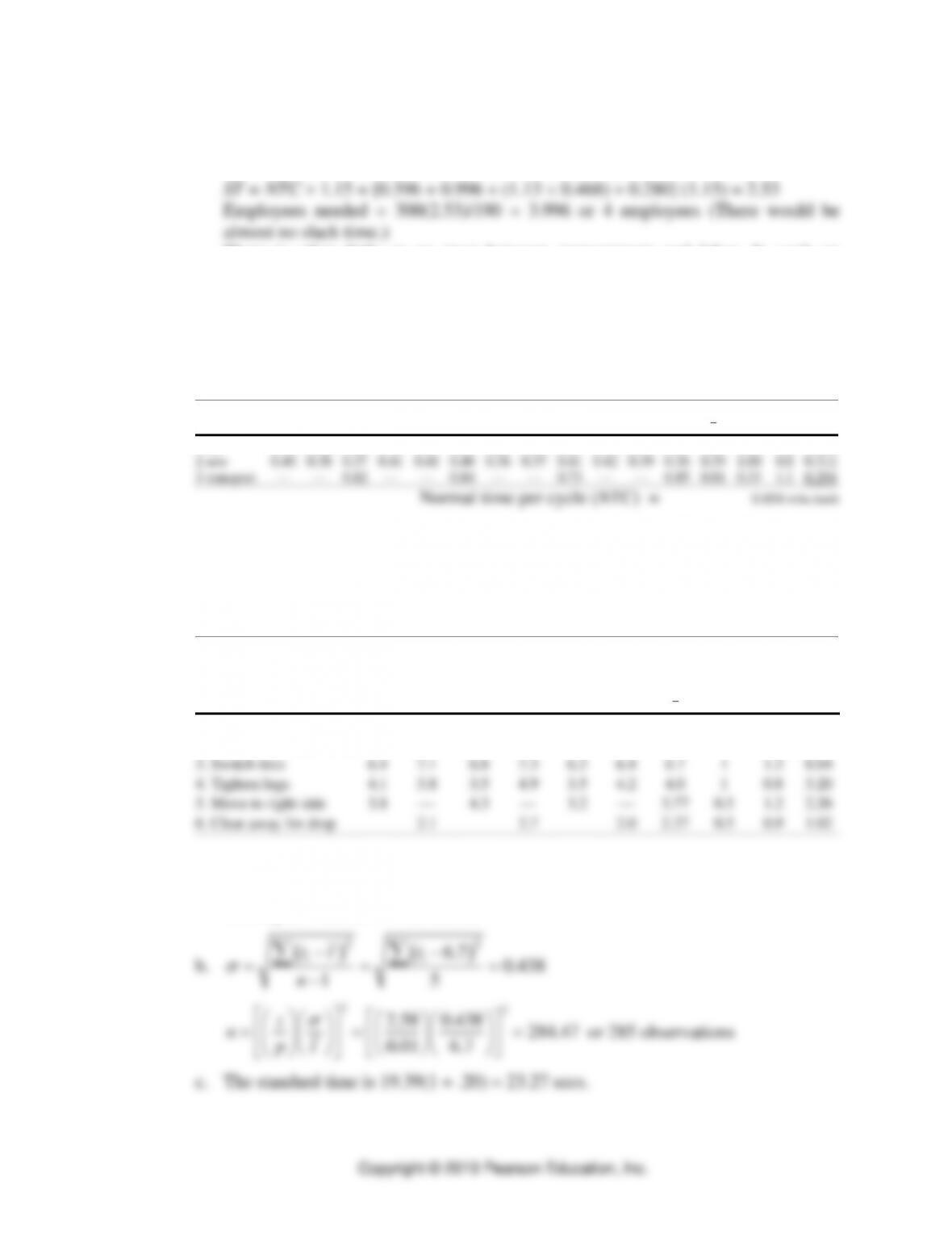
a. The normal time for changing four tires is 19.39 seconds. (A bit slow for a pit
stop. Apparently the Superfast Speedway still needs some improvement in order
to compete with the Woods Bros.)
⚫
SUPPLEMENT H Measuring Output Rates
⚫
H-4
7. Cellular telephone assembly
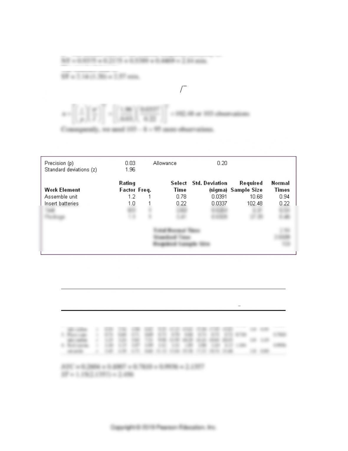
a. The normal time for the cellular telephone assembly is:
The standard time is:
b. The element with the largest value of
t
is “Insert batteries.” The required
sample size is:
22
1.96 0.0337 102.48 or 103 observations
z
These calculations are confirmed by the Time Study Solver of OM Explorer:
8. Coffee cup packaging
a. The select times, average times, and normal times for each work element are
shown in the following table.
Operation: COFFEE CUP PACKAGING
Date: 1/23
Operator: B. LARSON
Clock no: 43-6205
Element
Observations
Description
1
2
3
4
5
6
7
8
9
10
t
F
RF
NT
1. Get two
t
0.48
—
0.46
—
0.54
—
0.49
—
0.51
—
0.496
0.2604
cartons
r
0.48
4.85
9.14
13.53
17.8
0.5
1.05
2. Put liner
t
0.11
0.13
0.09
0.10
0.11
0.13
0.08
0.12
0.10
0.09
0.106
0.1007
into carton
r
0.59
2.56
4.94
6.82
9.25
11.23
13.61
15.50
17.93
19.83
1.0
0.95
3. Place cups
t
0.74
0.68
0.71
0.69
0.73
0.70
0.68
0.74
0.71
0.72
0.710
0.7810
into carton
r
1.33
3.24
5.65
7.51
9.98
11.93
14.29
16.24
18.64
20.55
1.0
1.10
4. Seal carton,
t
1.10
1.15
1.07
1.09
1.12
1.11
1.09
1.08
1.10
1.13
1.104
0.9936
set aside
r
2.43
4.39
6.72
8.60
11.10
13.04
15.38
17.32
19.74
21.68
1.0
0.90
NTC = 0.2604 + 0.1007 + 0.7810 + 0.9936 = 2.1357
ST = 1.15(2.1357) = 2.456
Measuring Output Rates
⚫
SUPPLEMENT H
⚫
H-5
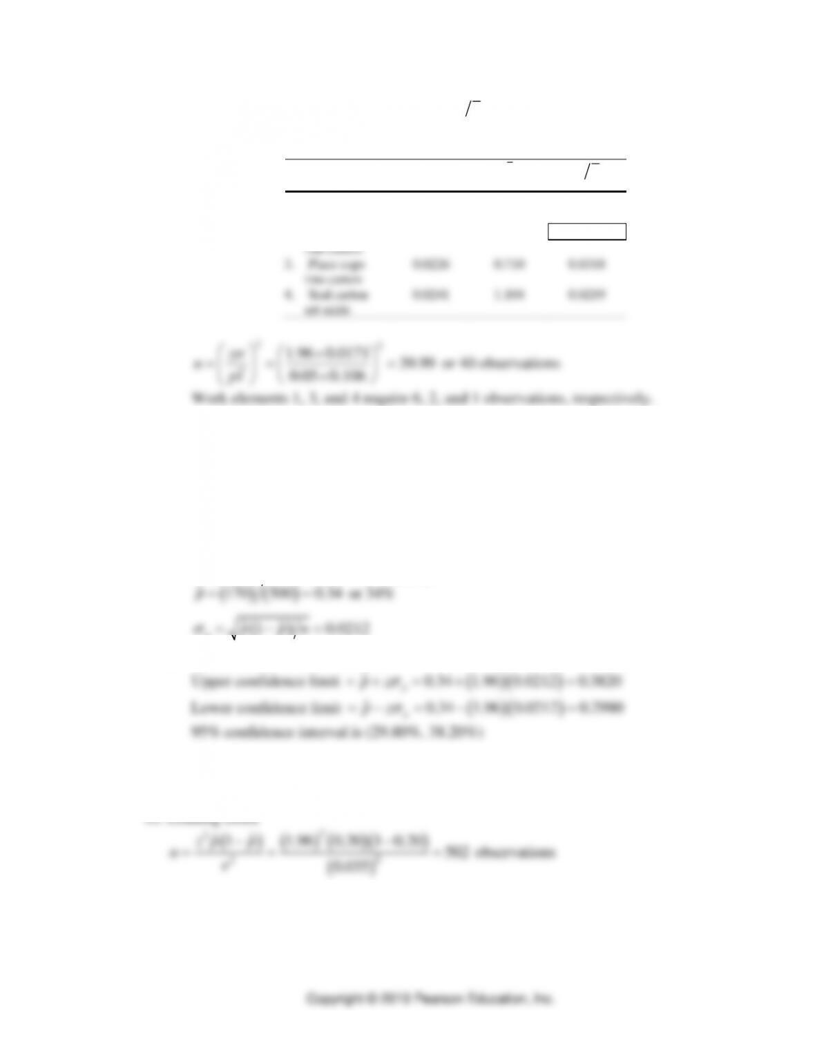
b. Because of the relatively high ratio
( )
t
for the second work element, it
requires more observations than do the other work elements.
Element
Description
t
t
1. Get two
0.0305
0.496
0.0615
Cartons
2. Put liner
0.0171
0.106
0.1613
into carton
3. Place cups
0.0226
0.710
0.0318
into carton
4. Seal carton
0.0241
1.104
0.0219
set aside
c. Doubling the precision interval reduces the required number of observations by a
factor of four. The number of observations required for 10% precision is 10. We
have already made enough observations for 95% confidence with a 10% precision
interval.
Work Sampling Method
9. Nurses’ Station
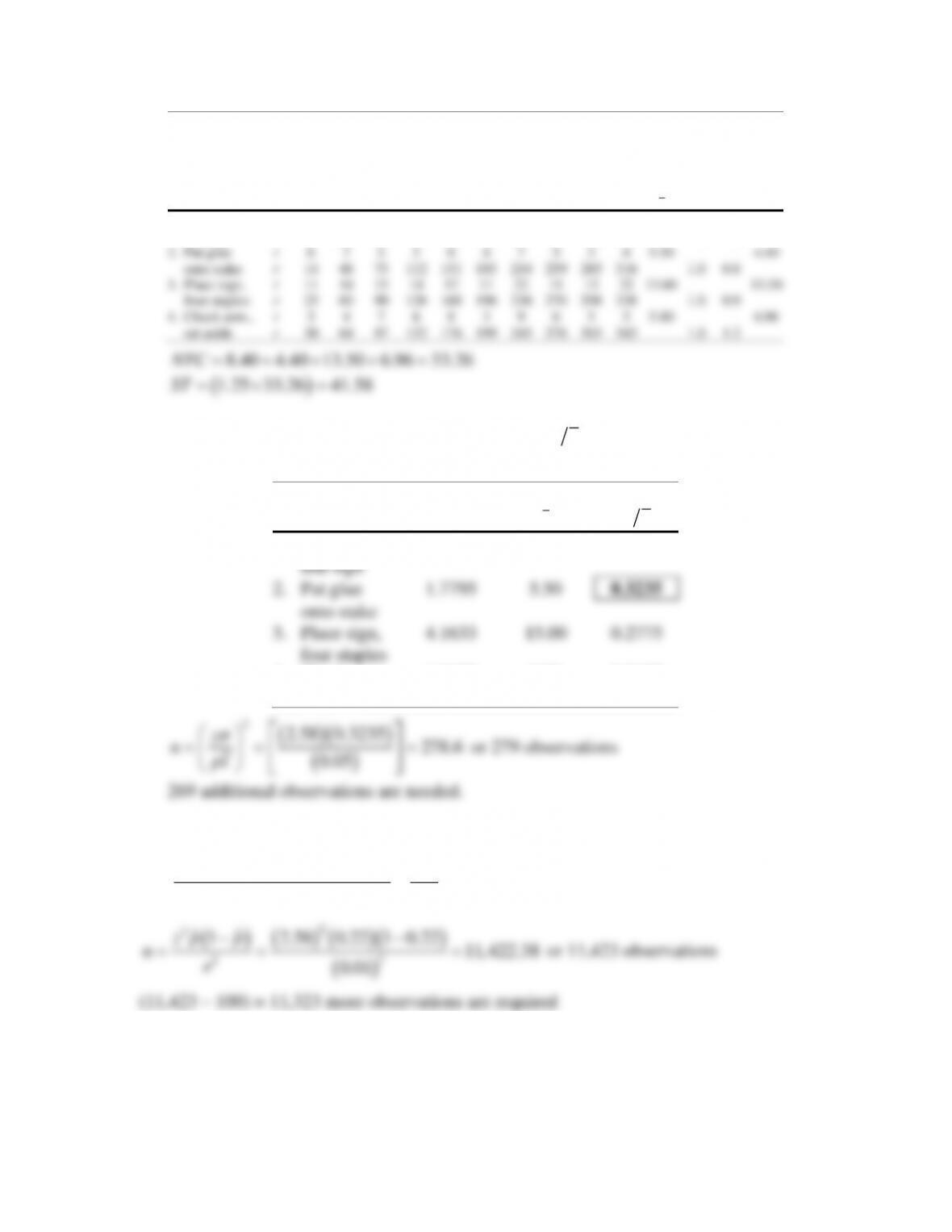
a. Proportion of time spent in doing paperwork
⚫
SUPPLEMENT H Measuring Output Rates
⚫
Copyright © 2019 Pearson Education, Inc.
H-6
Graft City
Form #
13-4927-R364
Public Works Department
James (Jimmy) Johnson, Director
Operation: YARD SIGN ASSEMBLY
Date 9/27
Observer: public works employee
Element
Observations
Description
1
2
3
4
5
6
7
8
9
10
t
F
RF
NT
1. Get stake
t
8
9
6
10
10
5
8
9
6
9
8.00
8.40
and sign
r
8
39
70
107
142
181
207
254
282
312
1.0
1.05
2. Put glue
t
6
7
5
5
9
4
7
5
3
4
5.50
4.40
onto stake
r
14
46
75
112
151
185
214
259
285
316
1.0
0.8
3. Place sign,
t
11
14
15
14
17
11
22
11
13
22
15.00
13.50
four staples
r
25
60
90
126
168
196
236
270
298
338
1.0
0.9
4. Check asm.,
t
5
4
7
6
8
3
9
6
5
5
5.80
6.96
set aside
r
30
64
97
132
176
199
245
276
303
343
1.0
1.2
b. The second work element has the highest ratio of
t
so it will require the most
observations.
Element
Description
t
t
1. Get stake
1.7638
8.00
0.2205
and sign
2. Put glue
1.7795
5.50
0.3235
onto stake
3. Place sign,
4.1633
15.00
0.2775
four staples
4. Check asm.,
1.8135
5.80
0.3127
set aside
12. Universal Life Insurance Company. The preliminary work sample provides an
estimate for the proportion of time data entry operator is idle.
2 3 3 4 1 3 6 2
ˆ0.22
13 15 14 16 14 16 12 100
p+ + + + + +
= = =
++++++
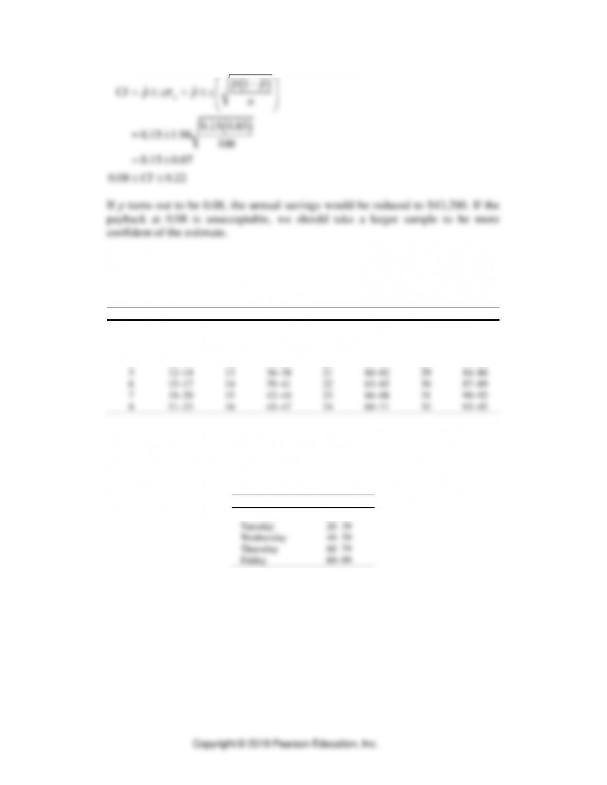
13. Valley Forge Post Office (assuming 95% confidence interval)
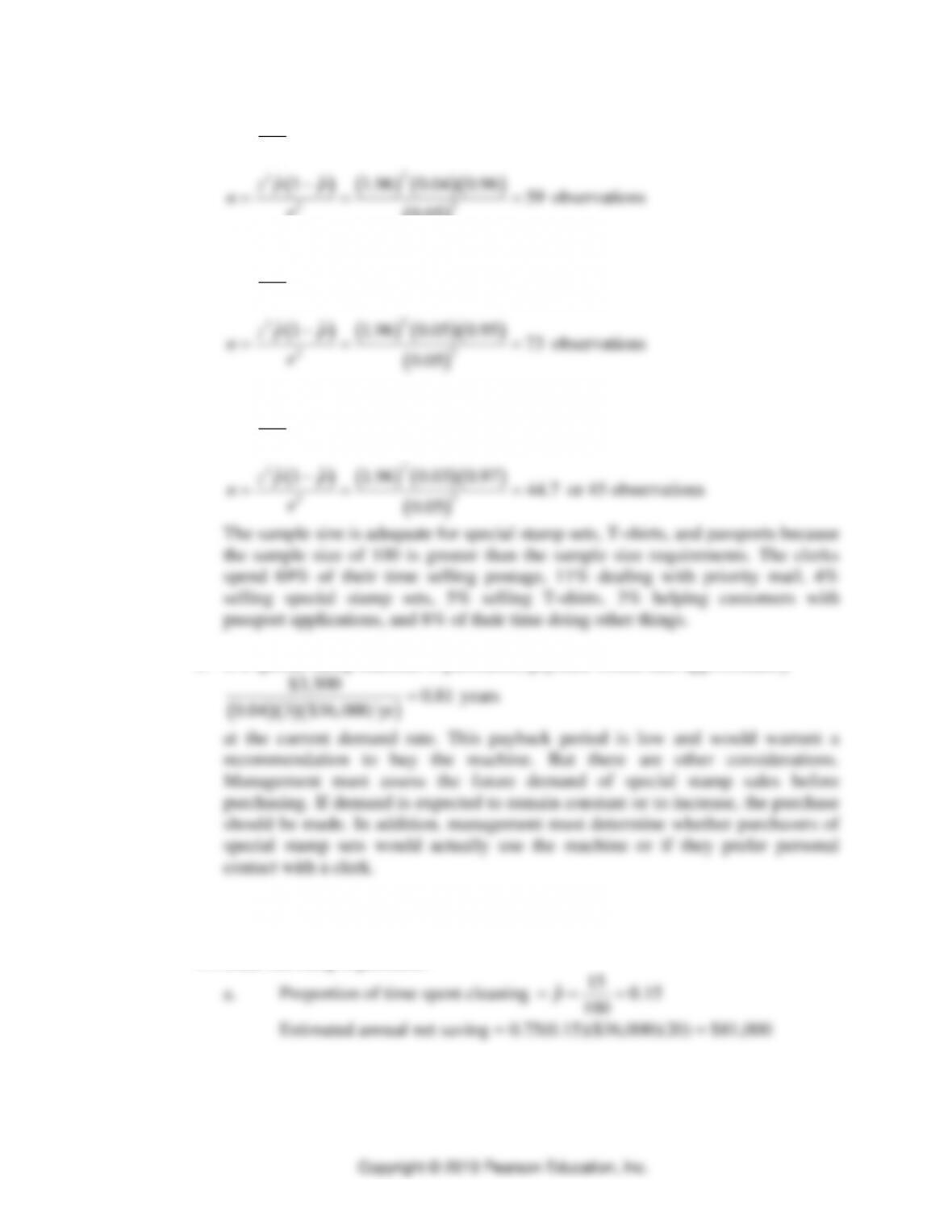
a. Special stamp sales
Measuring Output Rates
⚫
SUPPLEMENT H
⚫
H-7
4
ˆ0.04
100
p==
3
ˆ0.03
100
p==
⚫
SUPPLEMENT H Measuring Output Rates
⚫
H-8
( )
ˆˆ
1
ˆˆ
p
pp
CI p z p z n
−
= =
15. Machine shop work sampling
a. Because each day can be grouped into 32 15-minute periods (excluding lunch
time), the allocation of the 100 random numbers to these 32 periods is:
Period
RN
Period
RN
Period
RN
Period
RN
1
00–02
9
24–26
17
48–50
25
72–74
2
03–05
10
27–29
18
51–53
26
75–77
3
06–08
11
30–32
19
54–56
27
78–80
4
09–11
12
33–35
20
57–59
28
81–83
5
12–14
13
36–38
21
60–62
29
84–86
6
15–17
14
39–41
22
63–65
30
87–89
7
18–20
15
42–44
23
66–68
31
90–92
8
21–23
16
45–47
24
69–71
32
93–95
Note: Random numbers 96–99 will be discarded so that each period is assigned
equal probability, 3%.
Similarly, we can assign random numbers to the event “day,” each of which has a
probability of 20%.
Day
RN
Monday
00–19
Tuesday
20–39
Wednesday
40–59
Thursday
60–79
Friday
80–99
To generate two streams of 20 random numbers, the following procedures are
performed.
(1) Draw 20 random numbers from the first three rows of the table of random
numbers on page E-17 (supplement E) of the text. Start with the first number
in the first row, then go to the second number in the first row, and so on. For
each random number drawn, find the associated 15-minute period. Random
numbers 96–99 should be discarded.

Measuring Output Rates
⚫
SUPPLEMENT H
⚫
H-9
(2) Draw another 20 random numbers from rows 4, 5, and 6. Start with the first
number in row 3, then go to the second number in row 3, and so on. For each
random number drawn, find the associated day.
Accordingly, an observation schedule can be constructed.
Observation
Period
15-Minute
Observation
Period
15-Minute
Number
RN
Period
Number
RN
Period
1
71
24*
11
30
11
2
68
23
12
23
8
3
48
17
13
89
30
4
64
22
14
58
20
5
13
5
15
46
16
6
36
13
16
00
1
7
58
20
17
82
28
8
13
5
18
02
1
9
93
32
19
37
13
10
21
8
20
50
17
* For example, this period represents 2:45 P.M.–3:00 P.M.
Observation
Day
Observation
Day
Number
RN
Day
Number
RN
Day
1
31
2
11
01
1
2
77
4
12
27
2
3
58
3
13
19
1
4
59
3
14
36
2
5
23
2
15
05
1
6
25
2
16
42
3
7
37
2
17
20
2
8
44
3
18
76
4
9
92
5
19
54
3
10
42
3
20
03
1
⚫
SUPPLEMENT H Measuring Output Rates
⚫
H-10
b.
Observation
Time of
Observed
Number
Day
Day
Activity
1
24
2
I
2
23
4
R
3
17
3
R
4
22
3
B
5
5
2
R
6
13
2
R
7
20
2
S
8
5
3
R
9
32
5
R
10
8
3
B
11
11
1
R
12
8
2
R
13
30
1
R
14
20
2
R
15
16
1
R
16
1
3
I
17
28
2
R
18
1
4
S
19
13
3
R
20
17
1
B
R: Running; S = Setup; I = Idle; B = Breakdown
Activity
Proportion
Running
13/20 =
0.65
Setup
2/20 =
0.10
Idle
2/20 =
0.10
Breakdown
3/20 =
0.15
Total
1.00
c. The actual proportions of time spent on each activity are:
Activity
Proportion
Running
118/160 =
0.74
Setup
21/160 =
0.13
Idle
11/160 =
0.07
Breakdown
10/160 =
0.06
Total
1.00

Measuring Output Rates
⚫
SUPPLEMENT H
⚫
H-11
Except for the proportions of setup and idle time, the estimates are not very
accurate. The poor estimates may be attributed to small sample size, 20 in this
case. The sample sizes needed to ensure accuracy within ±0.04 with 95%
confidence for each activity may be determined using the formula
( )( )
2
2
1z p p
ne
−
=
.
Activity
Sample Size
Running
462
Setup
271
Idle
156
Breakdown
135
d. The sample size should be increased to 462 observations. This will ensure the
e. Currently, the estimates are not accurate due to small sample sizes. An increase