
Supplement
H Measuring Output Rates
1. Work Standards
• Work measurement as a management tool
o An essential input to managing processes and supply chains.
• Work standard: the time required for a trained worker to perform a task following a
prescribed method with normal effort and skill.
o How work standards are used:
▪ Establishing prices and costs
▪ Motivating workers
▪ Comparing alternative process designs
▪ Scheduling
▪ Capacity planning
▪ Performance appraisal
1. Developing a Work Standard: Key is to define normal performance.
2. Methods of Measuring Output Rates: Formal methods of work measurement, which is the
process of creating labor standards based on the judgment of skilled observers, include:
a. Time study method
b. Elemental standard data method
c. Predetermined data method
d. Work sampling method
2. Time Study Method
1. Time study is the method used most often for setting time standards.
a. Steps in a time study (Illustrate quickly with Examples H.1−H.3, and accompanying
PowerPoint slides.)
• Step 1. Selecting work elements—each should have definite starting and
stopping points. Separate incidental operations from the repetitive work.
• Step 2. Timing the elements—Use either the continuous or snap-back
method. Irregular occurrences should not be included in calculating the average
time.
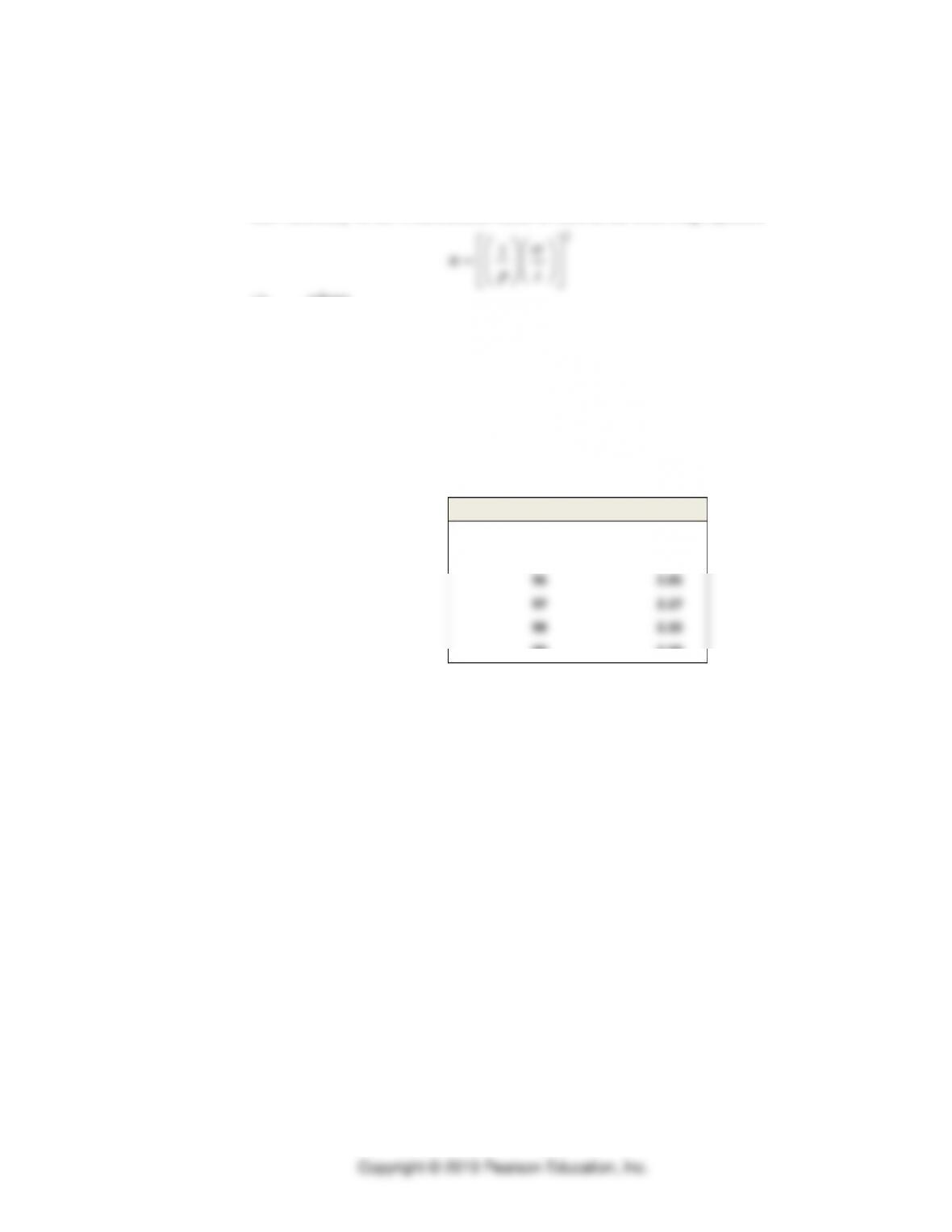
• Step 3. Determining sample size (n) which varies with confidence, precision,
and variability of the work element times as seen in the following equation
where
n = required sample size
p = precision of the estimate as a proportion of the true value
𝒕 ̅ = select time for a work element
σ = standard deviation of representative observed times for a work element
z = number of normal standard deviations needed for the desired confidence
Typical values of z for this formula are as follows:
Desired Confidence (%) z
90 1.65
95 1.96
96 2.05
97 2.17
98 2.33
99 2.58
Use Example H1: A coffee cup packaging operation, to practice sample size
calculations.
Tutor H.1 in MyLab Operations Management provides a new example to
practice the approach to determine the appropriate sample size.
• Step 4. Setting the standard—Apply subjective performance rating factor,
calculate normal times, normal time for the cycle, and adjust for allowances.
Tutor H.2 in MyLab Operations Management provides a new example to
practice the determination of the normal time.
Tutor H.3 in MyLab Operations Management provides a new example of
determining the standard time.
b. Use Application H.1 to give the students an opportunity to go through the four steps in
a time study on their own.
Lucy and Ethel have repetitive jobs at the candy factory. Management desires to
establish a time standard for this work for which they can be 95% confident to be within
± 6% of the true mean. There are three work elements involved:
Step 1: Selecting work elements.
#1: Pick up wrapper paper and wrap one piece of candy.
2
#2: Put candy in a box, one at a time.
#3: When the box is full (4 pieces), close it and place on conveyor.
Step 2: Timing the elements.
Select an average trained worker: Lucy will suffice.
Element
Initial Observation Cycle Number, Minutes
Select
Time,
t
Standard
Dev,
1
2
3
4
5
6
7
8
9
Wrap #1:
.10
.08
.08
.12
.10
.10
.12
.09
.11
Pack #2:
.10
.08
.08
.11
.06
.98*
.17
.11
.09
Close #3:
.27
…
…
…
.34
…
…
…
.29
* Lucy had some rare and unusual difficulties; don’t use this observation.
Step 3: Determining sample size.
First calculate
t
for each element in Step 2.
Element
Initial Observation Cycle Number, Minutes
Select
Time,
t
Standard
Dev,
1
2
3
4
5
6
7
8
9
Wrap #1:
.10
.08
.08
.12
.10
.10
.12
.09
.11
0.1
0.015
Pack #2:
.10
.08
.08
.11
.06
.98*
.17
.11
.09
0.1
0.03295
Close #3:
.27
…
…
…
.34
…
…
…
.29
0.3
0.03606
Next show the PowerPoint slide that shows the answers above. including each
element’s standard deviation (to save the students from calculating the standard
deviation because of time limitations).
Have students next determine the sample size, assuming a 95% confidence interval,
with z =1.96. The precision interval of ± 6% of the true mean implies p = 0.06.
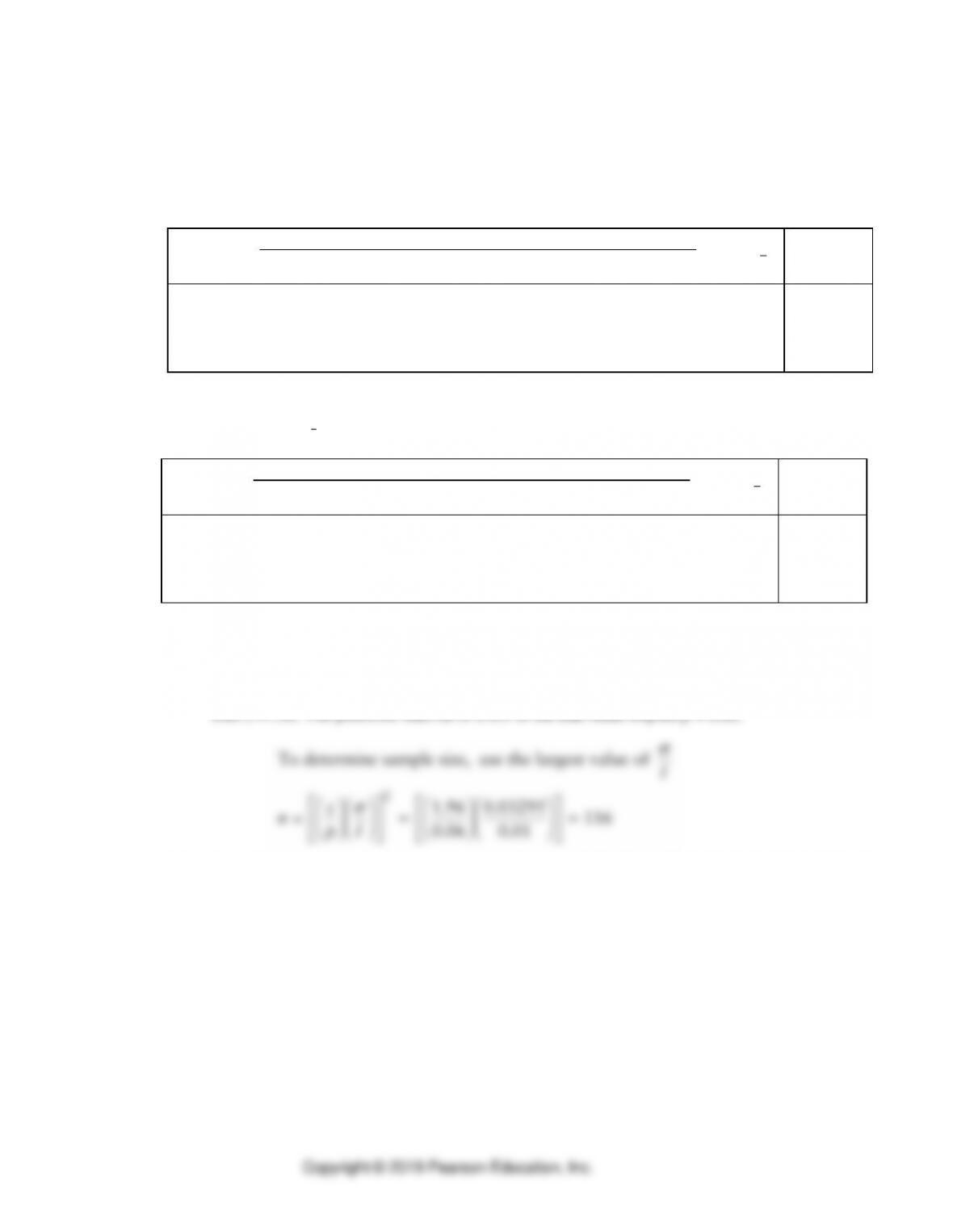
Step 4: Setting the standard.
a. The analyst subjectively assigns a rating factor (shown below).
b. Determine the normal time (NT) for each work element, given the following rating
factors. (Students complete highlighted sections)
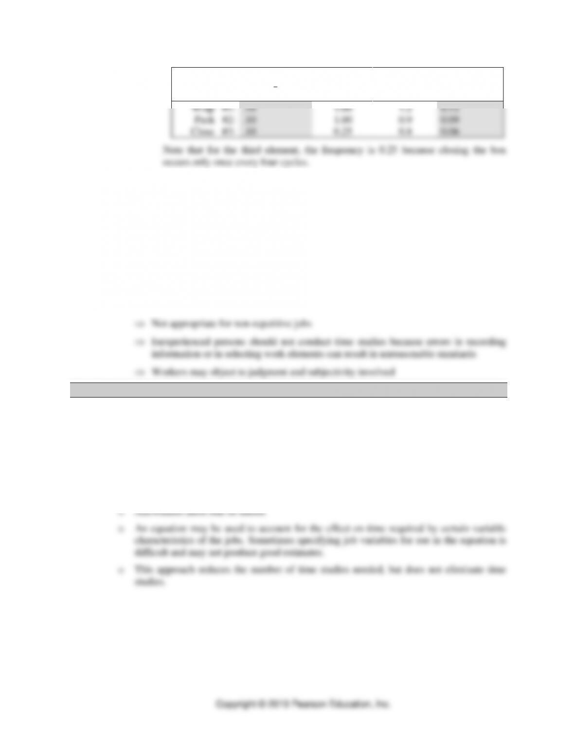
Element
Select Time,
t
Frequency
Rating
Factor
Normal
Time
Wrap #1:
.10
1.00
1.2
0.12
Pack #2:
.10
1.00
0.9
0.09
Close #3:
.10
0.25
0.8
0.06
Note that for the third element, the frequency is 0.25 because closing the box
occurs only once every four cycles.
c. Determine the normal time for the cycle. (0.27 minutes)
d. Subjectively determine the proportion of the normal time to be added for allowance,
and then calculate standard time ST. Let the allowances be 18.5% of the normal
time. (Adding the allowance gives a standard time of 0.32 minutes.)
c. Overall assessment of time study
• Most frequently used method for setting time standards
• Qualified analysts can typically set reasonable standards
Not appropriate for “thinking” jobs
3. Elemental Standard Data Method
• Useful for processes with high divergence, but when a high degree of similarity exists for basic
elements of work for different services and processes.
• The basic approach:
o Time standards are developed for common work elements.
o Study results are stored in a database for later use in establishing standards for jobs
requiring those elements.
4. Predetermined Data Approach
• Break each work element into micromotions: reach, move, disengage, apply pressure,
grasp, position, release, and turn.
• The basic approach:
o Step 1: Break each work element into its basic micromotions – reach, move,
disengage, apply pressure, grasp, position, release, and turn.
• Advantages of predetermined data approach:
o Standards can be set for new jobs.
o Work methods can be compared without a time study.
o Greater consistency of results, variation due to recording errors and difference
between workers is removed.
o Lessons the problem of biased judgment in performance rating.
• Disadvantages of predetermined data approach:
5. Work Sampling Method
• Estimates the proportion of time spent by people and machines on activities, based on a large
number of observations.
• Results in a proportion of time spent doing an activity, rather than a standard time for the
work.
o Requires a large number of random observations spread over the length of the
study.
o Proportion of observations in which the activity occurs is assumed to be the
proportion of time spent on the activity in general.
1. Work Sampling Procedure: Basic approach (Illustrate quickly with Example H.4, and
accompanying PowerPoint slides.)
a. Step 1. Define the activities.
b. Step 2. Design the observation form.
c. Step 3. Determine the length of the study.
d. Step 4. Determine the initial sample size.

e. Step 5. Select random observation times using a random number table.
f. Step 6. Determine observer schedule.
g. Step 7. Observe the activities and record the data.
h. Step 8. Decide whether further sampling is required.
2. Sample size: Select a sample size so that the estimate of the proportion of time spent on a
particular activity that does not differ from the true proportion by more than a specified error.
a. For the binomial distribution, the maximum error (e) of the estimate is:
Where:
pˆ
= sample proportion
e = maximum error in the estimate
n = sample size
z = standard deviations needed to achieve the desired confidence
• Use Application H.2 to see whether the students understand the work sampling
approach.
o Major League Baseball (MLB) is concerned about excessive game duration. Batters
now spend a lot of time between pitches when they leave the box to check signals
with coaches, and then go through a lengthy routine including stretching and a
variety of other actions. Pitching routines are similarly elaborate. In order to speed up
the game, it has been proposed to prohibit batters from leaving the box and to
prohibit pitchers from leaving the mound after called balls and strikes. MLB
estimates the proportion of time spent in these delays to be 20% of the total game
time. Before they institute a rules change, MLB would like to be 95% confident that
the result of a study will show a proportion of time wasted that is accurate within
±4% of the true proportion.
Steps 1 and 2. Define the activities and design the observation form.
Step 3. Determine the length of the study. Suppose that ten games (or 32 hours) are appropriate.
Step 4. Determine the initial sample size.
n =
æ
è
ç ö
ø
÷ 2
0.20 1 – 0.20
( )
=
Note to Instructor: The answer is 385 observations, using 20% as an initial estimate.
Steps 5 and 6. Determine the observer schedule.
Note to Instructor: You need 12 per hour to get 385 observations in 32 hours.
eppep +− ˆˆˆ
( )
n
pp
ze ˆˆ −
=1
Step 7. Observe the activities and record the data.
Note to Instructor: Suppose you find 96 unacceptable delays for pitcher and 46 unacceptable
delays for batters.
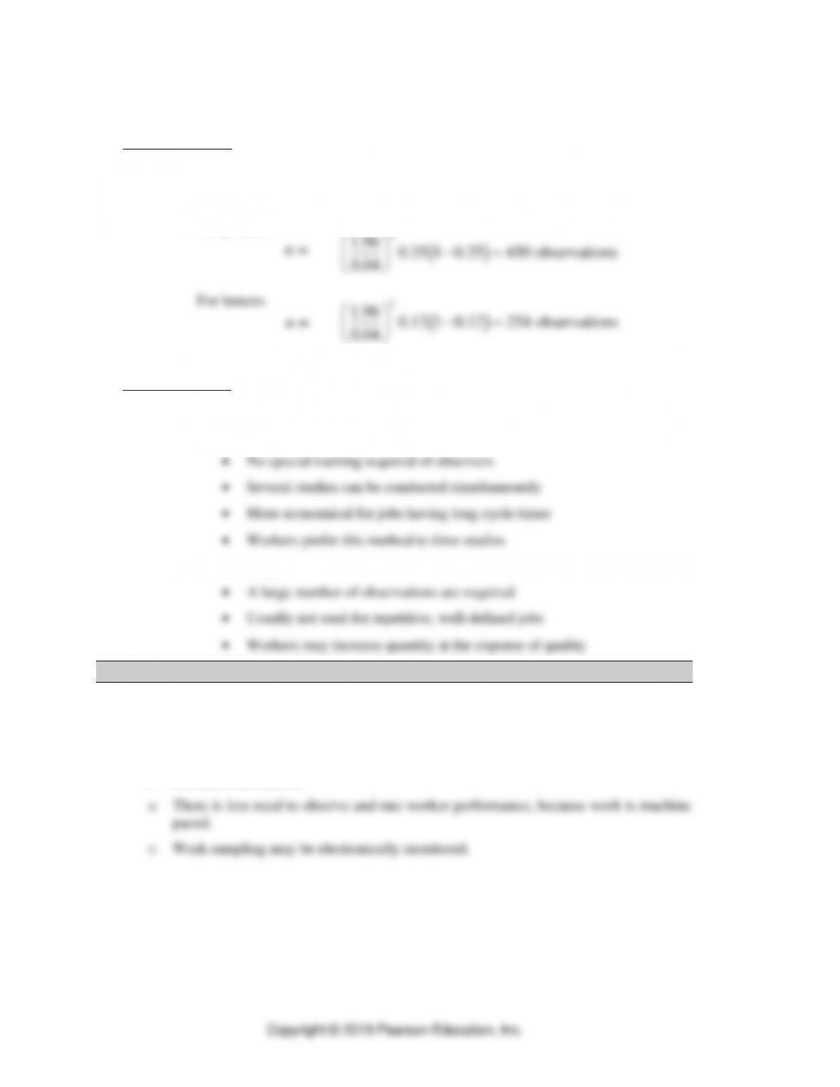
Step 8. Check to see whether additional sampling is required.
For pitchers:
0.04
2
1.96 0.12 1 0 25.12 observation4 s
Conclusion?
Note to Instructor: You need 65 more observations.
3. Overall assessment of work sampling
a. Advantages
b. Disadvantages
6. Managerial Considerations in Work Measurement
• Managers should carefully evaluate work measurement techniques to ensure that they are
used in ways that are consistent with the firm’s competitive priorities.
• Technological changes
o Increased automation
2
1.96 0.25 1 0 45.25 observation0 s
−=
0.04